Introduction
So far we’ve only been using fastai to train our models. But what exactly is happening under all the nice functions that we’ve learned to use? Well that’s what this post is about. We will take a look at the fundamental building blocks of neural network and create them from scratch using pure Python and PyTorch.
A problem with modeling with deep learning is, how complex does our model have to be? Make it too complex and the trade of of time vs accuracy is not worth it; make it too small and it will not perform well. But what exactly do we mean by perform well? Every deep learning project needs some form of a baseline which we can improve upon - sometimes this baseline is a human, sometimes a simple model. We will explore this idea in this post as well.
Our objective in this blog is to recognize handwritten digits with the very famous MNIST dataset. While building our own neural network, we will keep things simple and to the point. However, that comes at a cost of not implementing some of the tools that libraries implement to make model training as fast as possible. Therefore, in the process of building NN from scratch, we will look at a small subset of MNIST. Later on, we will use the entire dataset to use a pretrained model using fastai.
Classifying Handwritten Digits with a model from scratch
The MNIST dataset is a dataset with a lot of history behind it. It’s often used as a “Hello World” dataset to modeling based on deep learning. We will use a subset of the dataset containing only the digits “3” and “7”. Let’s get the MNIST_SAMPLE dataset that fastai provides. But before that, we will of course import required librar(ies).
from fastai.vision.all import *

path = untar_data(URLs.MNIST_SAMPLE)
path.ls() # contains a bunch of directories and files
> (#9) [Path('cleaned.csv'),Path('item_list.txt'),Path('trained_model.pkl'),Path('models'),Path('valid'),Path('labels.csv'),Path('export.pkl'),Path('history.csv'),Path('train')]

(path/'train').ls() # interested in the train directory
> (#2) [Path('train/7'),Path('train/3')]
We will grab all the images from the (path/'train') directory and maybe we can try to open one of them.
threes = (path/'train'/'3').ls().sorted()
sevens = (path/'train'/'7').ls().sorted()

im3_path = threes[1]
im3 = Image.open(im3_path)
im3
Nice, we have the data now. Let’s inspect it. But what does inspecting an image mean? Well images are made up of pixels i.e. a black-and-white image is just a matrix of shape width x height with values between 0-255; colored images also have a depth where the depth is usually the number of color channels like red-green-blue (RGB).
We can look at the pixel values of the images using numpy which is another very useful library for data science.
import numpy as np
np.array(im3)[4:10,4:10]

> array([[ 0, 0, 0, 0, 0, 0],
         [0, 0, 0, 0, 0,29],
         [ 0, 0, 0, 48, 166, 224],
         [ 0, 93, 244, 249, 253, 187],
         [ 0, 107, 253, 253, 230, 48],
         [ 0, 3, 20, 20, 15, 0]], dtype=uint8)
Now, before we start training a deep learning model, let’s find the simplest way to understand whether two images are the same - by comparing their pixels.
The Baseline: Pixel Similarity
Long story short what we want to do are the following:
- Put all the images of each type into a list
- Stack up all the images and normalize (the pixel values are expected to be between 0 and 1, so we will also divide by 255 here)
- Take the mean along the dimension of stacking
- Use some distance as a loss to quantify how close an image is to a 3 or 7
# importing PyTorch
import torch

seven_tensors = [tensor(Image.open(o)) for o in sevens]
three_tensors = [tensor(Image.open(o)) for o in threes]

# divide by 255 to normalize
stacked_sevens = torch.stack(seven_tensors, 0).float()/255
stacked_threes = torch.stack(three_tensors, 0).float()/255
stacked_threes.shape
> torch.Size([6131, 28, 28])
SIDE NOTE: We will be working with tensors a lot. So, it’s good to know some basic terminology. Tensors are generalized matrices which is to say a matrix is a type of tensor. More specifically, matrices are rank-2 tensors. Given a tensor, t we can get its shape using t.shape which is the length of the tensor along every dimension. To get the rank of the tensor we use t.ndim.
Now that we have the stacked tensors, let’s take the mean along the dimension of stacking i.e. calculate what an average of all the 3s in our dataset looks like as well as a 7.
mean3 = stacked_threes.mean(0)
mean7 = stacked_sevens.mean(0)
Now to define a distance metric we have many different choices. We will stick to something very simple called the mean absolute deviation or mean absolute error (MAE) which is also known as L1 norm. The other choice is very similar called the mean square error (MSE) or L2 norm. \[ MAE = \frac{\sum_{i=1}^{m}|mean - x_i|}{\sum_{i=1}^{m}1} = \frac{1}{m}\sum_{i=1}^{m} |mean - x_i| \] \[ MSE = \frac{\sum_{i=1}^{m} (mean - x_i)^2}{\sum_{i=1}^{m}1} = \frac{1}{m}\sum_{i=1}^{m} (mean - x_i)^2 \]
We do this calculation in python using:
a_3 = stacked_threes[1]

dist_3_abs = (a_3 - mean3).abs().mean()
dist_3_sqr = ((a_3 - mean3)**2).mean().sqrt()

dist_3_abs,dist_3_sqr

> (tensor(0.1114), tensor(0.2021))
dist_7_abs = (a_3 - mean7).abs().mean()
dist_7_sqr = ((a_3 - mean7)**2).mean().sqrt()
dist_7_abs,dist_7_sqr
> (tensor(0.1586), tensor(0.3021))The smaller the distance the closer it is to the actual mean. With MSE, the errors bigger errors are penalized more as we square them. We can do this with PyTorch as well.
import torch.functional as F

F.l1_loss(a_3.float(),mean7), F.mse_loss(a_3,mean7).sqrt()

> (tensor(0.1586), tensor(0.3021))
There’s a very important section on the idea of broadcasting in the book. I will not cover that in this post as it is not the main focus of this. However, that being said, in the words of Jeremy:
It’s the most important technique for you to know to create efficient PyTorch code.
Take a look at that section in the book or somewhere online.
Stochastic Gradient Descent (SGD)
SGD is a cornerstone of the deep learning process. This is the step that allows us to nudge our loss function to a minimum value by changing weights. The four most common steps of training a model are:
Initialize: Initialize the weights in some random way as they will be updated anyway. However, certain ways of initialization is much better than others as we will see in the future.
Loss: This is the way we test the effectiveness of any current weight assignment in terms of actual performance. We need a function that will return a number that is small if the performance of the model is good and a large number if it’s bad.
Step: Stepping is the step where we update the weights using gradients. This is our optimization step and we can do it in several ways, one which happens to be stochastic gradient descent (SGD).
Stop: You can stop after some number of iterations in the learning process (epoch) or something like early stopping where you stop once the loss stops going down by a lot of the accuracy starts dropping again. There are many ways to deal with stopping the training.
Let’s take a look at a complete loop of these four steps.
Example end-to-end SGD
Let’s use some synthetic data. Add some noise and start there.
time = torch.arange(0,20).float()
speed = torch.randn(20)*3 + 0.75*(time-9.5)**2 + 1
When it comes to deep learning, we have to be careful about separating our input parameters from our parameter parameters i.e. the ones we want to change. Let’s also define our mse loss that calculates how well our predictions are.
def f(t, params):
   a,b,c = params
   return a*(t**2) + (b*t) + c


def mse(preds, targets): return ((preds-targets)**2).mean()
Now we have to do our steps:
- Initialize the weights
params = torch.randn(3).requires_grad_()requires_grad_() tells PyTorch that we want to calculate gradients with respect to these values. The _ at the end means it’s an inplace operation.
- Calculate the predictions
preds = f(time, params)- Calculate the initial loss
loss = mse(preds, speed)- Calculate the gradient of loss wrt the params
The gradient will give an approximation of how the parameters need to change:
loss.backward()
params.grad

> tensor([-53195.8594,  -3419.7146,   -253.8908])
A more indepth explanation of gradients and derivatives are explained in the book. In addition the playlist by 3Brown1Blue on Neural Networks does an incredible job at visualizing some of the core concepts of deep learning. Take a look at it here: https://youtube.com/playlist?list=PLZHQObOWTQDNU6R1_67000Dx_ZCJB-3pi.
- Step towards lower loss using the scaled gradients
Taking a step here means changing the weights by a scaled amount in the direction of the gradients we found in the previous step. The scaling factor is called the learning rate. We need to scale our gradients before we take a step because they are too large. Taking incredibly large steps might mean we miss our minima. However, if the learning rate is too small, we will also need a lot of time to converge. Therefore, this is a great topic of research. What is the best possible way to set a learning rate? Does it have to be a constant? What if we vary it over our iterations? These are things we will talk about in the future. For now, let’s say it should be a fairly small number like \(1 \cdot 10^{-5}\).
lr = 1e-5
params.data -= (lr * params.grad.data)
params.grad = None
There’s some odd things going on here in the code that we haven’t discussed yet. Why do we need params.data? Why can’t we just use params? What is up with setting the gradients to None? These are more so PyTorch implementation details that are quite important to know.
Once you tag a parameter with requires_grad_() PyTorch tends to calculate the gradients for every operation. Using params.data is the params tensor but with requires_grad = False. This way we do not calculate the gradients. In addition, PyTorch by default accumulates the gradients on every calculation i.e. if you do not set the gradients to 0 after a step, the next time your gradients will be the sum of the previous step and the current gradient. Usually we do not want that so we set params.grad = None or params.grad = 0 or params.grad.zero_.
- Run a loop n times
Let’s combine all the steps so far into a function and then run it n times.
def apply_step(params, prn = True):
  preds = f(time, params)
  loss = mse(preds, speed)
  loss.backward()
  params.data -= (lr * params.grad.data)
  params.grad = None
  if prn: print(loss.item())
  return preds

n = 10
for _ in range(n): apply_step(params)

> 5435.53662109375
  1577.4495849609375
  847.3780517578125
  709.22265625
  683.0757446289062
  678.12451171875
  677.1839599609375
  677.0025024414062
  676.96435546875
  676.9537353515625
As you can see, the loss is slowly going down.
- Stop
We decided to stop the training process after \(n=10\) steps. This was an arbitrary choice and you have a lot of freedom in choosing when to stop and based on what criteria. In practice, we would watch the training and validation losses and our metrics to decide when to stop, as we’ve discussed.
Training setup for MNIST problem
Let’s get back to our original problem of classifying digits. Now that we have looked at a simple example, we need to apply those same concepts to our problem.
Getting the data in the right representation
We want to have one large matrix of inputs and one large vector of labels. So, let’s stack the three and seven data.
train_x = torch.cat([stacked_threes, stacked_sevens]).view(-1, 28*28)
train_y = tensor([1]*len(threes) + [0]*len(sevens)).unsqueeze(1)
dset = list(zip(train_x,train_y))
.view(-1, 28*28) here is reshaping our stacked tensor so that each item has a (28 x 28) tensor. The -1 is an important thing to know. It tells PyTorch to calculate the remaining dimension’s size automatically. dset is now a list of tuples of x and y which we will feed to our neural network.
Do the same for the validation set.
valid_x = torch.cat([valid_3_tens, valid_7_tens]).view(-1, 28*28)
valid_y = tensor([1]*len(valid_3_tens) + [0]*len(valid_7_tens)).unsqueeze(1)
valid_dset = list(zip(valid_x,valid_y))
Initialization
We have to initialize our parameters (weights and biases) with some random values. It has been found that weight initialization is an incredibly important topic to train neural networks well. Here we use a very simple method but in the future we will look at some more advanced and better techniques for initialization.
def init_params(size, std=1.0):
  return (torch.randn(size)*std).requires_grad_()
weights = init_params((28*28,1))
bias = init_params(1)
The shapes of the matrices are very important as we will be performing matrix multiplication in the next section. It’s crucial to have a good understanding of how your data is being represented so you can initilize your parameters with the right shape!
Prediction
The prediction step in neural networks is a matrix multiplication. You’ll see people writing the steps in a few ways and the order of X and W depends on the shapes of the two tensors. In order for matrix multiplication to be valid, given X has shape (m, n), W must have the shape (n, k) and the resulting matrix will have shape (m, k). We can use the idea of a matrix transpose to also ensure that the orders are correct i.e. if W has shape (n, k), then \(W^{T}\) will have shape (k, n)
\[ \text{preds} = XW^{T} + b \]
In code we leverage the power of broadcasting to make our lives a little simpler.
def linear1(xb):
  # @ operator is for matrix multiplication
  return xb@W.T + b

preds = linear1(train_x)
We can get a very crude sense of accuracy. To decide if an output represents a 3 or a 7, we can just check whether it’s greater than 0.
corrects = (preds > 0).float() == train_y
corrects.float().mean().item()
Because this is binary classification in some sense we are essentially asking if the prediciton is a 3 or not (greater than 0 or not) and checking with the labels in train_y. Then we can average over how many were correct. In Python, True has a value of 1 and False 0.
Now, we should NOT use accuracy as a loss function as it does not have nice derivatives. The accuracy function is essentially a constant except at the threshold of 0.5. So, the derivatives are either 0 or undefined. Let’s see what we can choose as our loss function next.
Defining a loss
The first thing to understand is the closer the prediction is to our target, the lower the loss should be. So, if we can check how far our prediction is from 1, we should have a good loss function.
def mnist_loss(preds, targets):
  return torch.where(targets == 1, 1 - preds, preds).mean()
torch.where(a, b, c) says where a is True, use b else use c. So, wherever the target is 1, we are subtracting how far the prediction is from 1, else we are just using the prediction. Then we can the mean over everything.
mnist_loss(tensor([0.9, 0.4, 0.8]),trgts)
> tensor(0.2333)
Now, the problem here is we expect the predictions to always be between 0 and 1. But, right now, there is nothing bounding our predictions in that range. To do so, we have to wrap our predictions is some other function so the final output is bound between 0 and 1.
This is where the Sigmoid function comes into play.
def sigmoid(x):
  return 1/(1+torch.exp(-x))
Plotting this function gives us a function called the sigmoid function that is bound between 0 and 1 for all values of the input, x. 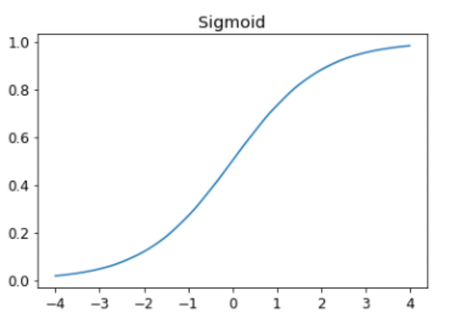
Let’s update our mnist_loss() function.
def mnist_loss(preds, targets):
  preds = preds.sigmoid()
  return torch.where(targets == 1, 1 - preds, preds).mean()
Loss and Metric
It’s very important at this stage to separate the concepts of loss vs metric.
LOSS: A loss is something we care about to automate our learning process. That is what we are trying to minimize to get the best weights. The loss function is calculated for each item in our dataset, and then at the end of an epoch, the loss values are all averaged and the overall mean is reported for the epoch.
METRIC: Metrics, on the other hand, are the numbers that we care about. It is used to drive human understanding of our the performance of the model.
SGD and Minibatches
With data and a choice of loss function, we are now ready for the optimization step. This is where we update the weights based on the gradients.
To take an optimization step, we need to calculate the loss over one or more data items. The question is how many points should we use? It’s been found that using too little is slow because we don’t use the full potential of our GPU as well as the learning process being too unstable, but using too much of the data can also lead to problems like we cannot fit the data into our GPU VRAM.
If the extremes don’t work, the best option is probably to use a subset of the data. We call these subsets, mini-batches and the number of data points in each mini-batch the batch size. A larger batch size means that you will get a more accurate and stable estimate of your dataset’s gradients from the loss function, but it will take longer, and you will process fewer mini-batches per epoch. Choosing a good batch size is one of the decisions you need to make as a deep learning practitioner to train your model quickly and accurately.
Augmentations, Randomization, and DataLoaders
Varying the data during training often results in better performance. We have already talked about this before when we trained our bear classifier in Lesson-2 blog. This is where augmentations come into play usually. But there are more ways to vary the data during training. One simple and effective thing we can vary is what data items we put in each mini-batch.
Rather than simply enumerating our dataset in order for every epoch, instead what we normally do is randomly shuffle it on every epoch, before we create mini-batches. PyTorch and fastai provide us with objects called Dataloaders that do that for us. They handle the process of shuffling and coalition of mini-batches.
A DataLoader can take any Python collection and turn it into an iterator over many batches. But for training we don’t want any plain old collection, we want a collection of tuples of independent and dependent variables.
A collection of tuple of independent and dependent variables in PyTorch is known as a Dataset. When we pass a Dataset to a DataLoader we will get back many batches that are themselves tuples of tensors representing batches of independent and dependent variables.
Let’s create a dummy Dataset and DataLoader:
ds = L(enumerate(string.ascii_lowercase))
# looks like: [(0, 'a'), (1, 'b'), ...]

dl = DataLoader(ds, batch_size = 6, shuffle = True)
# setting shuffle to be True randomizes the order of the data in each epoch
list(dl)
> [(tensor([17, 18, 10, 22,  8, 14]), ('r', 's', 'k', 'w', 'i', 'o')),
    (tensor([20, 15,  9, 13, 21, 12]), ('u', 'p', 'j', 'n', 'v', 'm')),
    (tensor([ 7, 25,  6,  5, 11, 23]), ('h', 'z', 'g', 'f', 'l', 'x')),
    (tensor([ 1,  3,  0, 24, 19, 16]), ('b', 'd', 'a', 'y', 't', 'q')),
    (tensor([2, 4]), ('c', 'e'))]
We are now ready to write our first training loop for a model using SGD!
First model: Linear model
Time to create our first model. Remember the steps:
- Data representation and DataLoader
- Initialization of weights
- Loss function
- Optimization step
- Train
We already have a Dataset so let’s create DataLoaders for training and validation.
dl = DataLoader(dset, batch_size=256)
valid_dl = DataLoader(valid_dset, batch_size=256)
Let’s define our model and initialize the weights.
import torch.nn

linear_model = nn.Linear(28*28,1)
w, b = linear_model.parameters()
In this case we are using the nn.Linear() from PyTorch which under the hood initializes the weights and defines a linear layer like we have been doing. Every PyTorch module knows what trainable parameters it has. That’s what linear_model.parameters() returns.
We have our choice of loss function. Let’s remind ourselves what it is:
def mnist_loss(preds, targets):
  preds = preds.sigmoid()
  return torch.where(targets == 1, 1 - preds, preds).mean()
Now we can start optimizing the weights over many epochs. The optimizer has two reponsibilities: it updates the weights which is called the step and it zeros the gradients afterwards. Let’s write a small class for this.
class BasicOptim:
  def __init__(self, params, lr):
    self.params = list(params)
    self.lr = lr

  def step(self, *args, **kwargs):
    for p in self.params:
      p.sub_(p.grad * lr)

  def zero_grad(self, *args, **kwargs):
    for p in self.params:
      p.grad = None
Let’s train!
def calc_grad(xb, yb, model):
  preds = model(xb)
  loss = mnist_loss(preds, yb)
  loss.backward()

def batch_accuracy(preds, targets):
  preds = preds.sigmoid()
  correct = (preds>0.5) == targets
  return correct.float().mean()


def validate_epoch(model):
  # put all the accuracies of the validation dataset in a list
  accs = [batch_accuracy(model(xb), yb) for xb,yb in valid_dl]

  # stack them take the mean and round to 4 decimal places and return
  return round(torch.stack(accs).mean().item(), 4)


opt = BasicOptim(linear_model.parameters(), lr)
def train_epoch(model, lr, params):
  for xb, yb in dl:
    calc_grad(xb, yb, model)
    opt.step()
    opt.zero_grad()


def train_model(model, epochs):
  for i in range(epochs):
    train_epoch(model)
    print(validate_epoch(model), end=' ')


train_model(linear_model, 20)
fastai makes already provides us with a bunch of these so we don’t have to write them from scratch every time.
E.g. SGD in fastai is the same as the BasicOptim we wrote.
linear_model = nn.Linear(28*28,1)
opt = SGD(linear_model.parameters(), lr)
train_model(linear_model, 20)
It provides us with Learner.fit which can be used in place of train_model(). But first we need to create a DataLoaders instance. We do this by passing in our training and validation DataLoader.
dls = DataLoaders(dl, valid_dl)We’ve used Learner before but mostly the vision application learner, vision_learner(). If we want to use a non-application learner, we need to give it a few more parameters like the optimizer and the loss function. We also use Learner.fit() instead of .fine_tune() since our model is not pretrained.
learn = Learner(dls, nn.Linear(28*28,1), opt_func=SGD, loss_func=mnist_loss, metrics=batch_accuracy)
learn.fit(10, lr=lr)
Second model: Adding Non-Linearity
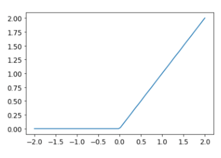
We can do even better than what we have by building deeper and more complex models. One thing to keep in mind before that is, a sum of linear functions is just a bigger linear function. That is to say if we don’t add any non-linearity to our model, we will not really increase its complexity in a meaningful way. The way we add non-linearity is by passing what we have been calling preds through activation functions. There are many that are out there but by far the most common is the rectified linear unit, ReLU. Passing anything through a ReLU ensures that it’s always non-negative.
\[ ReLU(x) = \max(0, x) \]
Let’s use PyTorch’s tools to create a model with 1 hidden layer (so input, 1 hidden, and then output layers) with some non-linearity!
simple_net = nn.Sequential(
  nn.Linear(28*28, 30),
  nn.ReLU(),
  nn.Linear(30, 1)
)
nn.Sequential() sets up the layers and computes predictions through the layers just like we have done so far.
Let’s use a Learner to fit.
learn = Learner(dls, simple_net, opt_func=SGD,
                loss_func=mnist_loss, metrics=batch_accuracy)

learn.fit(40, 0.1)
Accuracy over the epochs
The training process is recorded in learn.recorder, with the table of output stored in the values attribute, so we can plot the accuracy over training and also get the final accuracy:
plt.plot(L(learn.recorder.values).itemgot(2));

learn.recorder.values[-1][2]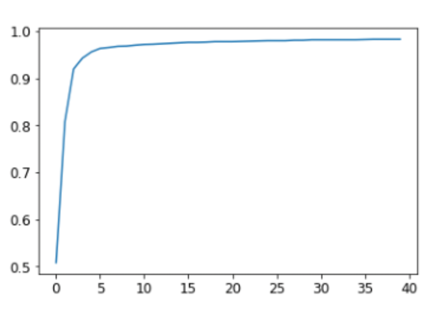
This is great. We have taken the first steps in learning how to create and train a neural network from scratch. Now, all we will be learning are ways to make these stes faster and better. The deeper the model gets, the harder it is to optimize the parameters in practice and we need to learn how to handle these problems soon.
Classifying Handwritten Digits with FastAI
The code is very similar to what we have done so far. I will not provide much explanation for it as it is almost entirely similar. The goal of this exercise was to see if I could repeat those steps from memory.
from fastai.vision.all import *
from fastai.vision.widgets import *
from fastcore.all import *


path = untar_data(URLs.MNIST)
test_path, train_path = path.ls()[0], path.ls()[1]


dblock = DataBlock(
    blocks = (ImageBlock, CategoryBlock),
    get_items = get_image_files,
    get_y = parent_label,
    splitter = RandomSplitter(valid_pct = 0.2),
    batch_tfms = [*aug_transforms(),
                 Normalize.from_stats(*imagenet_stats)]
)

dls = dblock.dataloaders(train_path, bs=32)

learn = vision_learner(dls, 'resnet34', metrics=error_rate)

lr = learn.lr_find()
learn.fine_tune(epochs=3, base_lr=lr.valley)

learn.export('mnist_resnet34.pkl')
The only new pieces of code here that we have not seen so far are:
Normalize.from_stats(*imagenet_stats): We normalize our models to train faster. In this specific case, we are using a pretrained modelresnet34as a result we need to normalize our data based on what the model was trained on. The*imagenet_statsis what ensures that the model is normalized with the same mean and standard deviation as the ImageNet dataset.lr = learn.lr_find(): So far we were just randomly choosing a learning rate. We can do better.lr_find()is a nice function that thefastailibrary provides for us to get a better suggestion for our lr. There are more advanced ways of controlling the learning rate that we will learn much later! More