From Dogs and Cats to Pet Breeds
In real life we start with a dataset that we know nothing about. We then have to figure out how it is put together, how to extract the data we need from it, and what that data looks like. Let’s use the PETS dataset.
from fastai.vision.all import *

path = untar_data(URLs.PETS)
Data is usually provided in one of these two ways:
Individual files representing items of data, such as text documents or images, possibly organized into folders or with filenames representing information about those items
A table of data (e.g., in CSV format) in which each row is an item and may include filenames providing connections between the data in the table and data in other formats, such as text documents and images.
Let’s see what our data looks like.
path.ls()We can see that this dataset provides us with images and annotations directories. We only need the images for classification (annotations are for localization).
(path/"images").ls()The labels of the breed are present in these filenames. We will use a regular expression to extract that. Let’s use the findall method to try a regular expression against the filename of the fname object:
re.findall(r'(.+)_\d+.jpg', (path/"images").ls()[0].name)This regex will give us all the characters leading up to the last underscore character, as long as the subsequent characters are numerical digits and then the JPEG file extension.
Let’s create the dataloaders.
dblock = DataBlock(
  blocks = (ImageBlock, CategoryBlock),
  get_items = get_image_files,
  get_y = using_attr(RegexLabeller(r'(.+)_\d+.jpg'), 'name'),
  splitter = RandomSplitter(seed=42),
  item_tfms = [Resize(460)],
  batch_tfms = [*aug_transforms(size=224, min_scale=0.75))]
)

dls = dblock.dataloaders(path/'images')
Presizing
The item_tfms and batch_tfms contain resizing operations. This is because we need our images to fit in our GPU. However, resizing down to the augmented size and other augmentation transforms introduce empty zones, degraded data, etc. This is why presizing can be extremely helpful. Presizing adopts two strategies:
Resize images to relatively “large” dimensions—that is, dimensions significantly larger than the target training dimensions.
Compose all of the common augmentation operations (including a resize to the final target size) into one, and perform the combined operation on the GPU only once at the end of processing, rather than performing the operations individually and interpolating multiple times.
The first step, the resize, creates images large enough that they have spare margin to allow further augmentation transforms on their inner regions without creating empty zones. This transformation works by resizing to a square, using a large crop size. On the training set, the crop area is chosen randomly, and the size of the crop is selected to cover the entire width or height of the image, whichever is smaller. In the second step, the GPU is used for all data augmentation, and all of the potentially destructive operations are done together, with a single interpolation at the end.
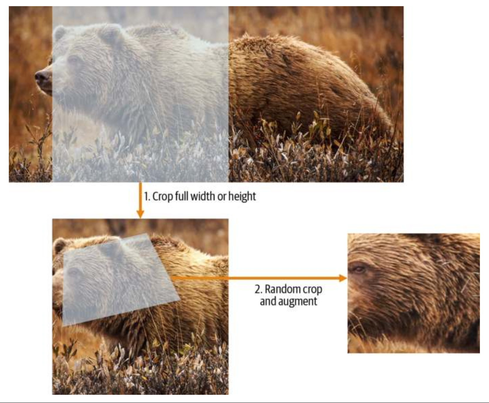
The picture above shows the two steps:
Crop full width or height: This is in item_tfms, so it’s applied to each individual image before it is copied to the GPU. It’s used to ensure all images are the same size. On the training set, the crop area is chosen randomly. On the validation set, the center square of the image is always chosen.
Random crop and augment: This is in batch_tfms, so it’s applied to a batch all at once on the GPU, which means it’s fast. On the validation set, only the resize to the final size needed for the model is done here. On the training set, the random crop and any other augmentations are done first.
To implement this process in fastai, you use Resize as an item transform with a large size, and RandomResizedCrop as a batch transform with a smaller size. RandomResizedCrop will be added for you if you include the min_scale parameter in your aug_transforms function.
Checking and Debugging a DataBlock object
Writing a DataBlock is like writing a blueprint. You will get an error message if you have a syntax error somewhere in your code, but you have no guarantee that your template is going to work on your data source as you intend. So, before training a model, you should always check your data.
There are two ways to debug a datablock object:
- Use
DataLoaders.show_batch()to see what the items in your batch look like. This can show you whether your items are labeled properly or if there arer mistakes. DataBlock.summary(). It will attempt to create a batch from the source you give it, with a lot of details. Also, if it fails, you will see exactly at which point the error happens, and the library will try to give you some help. It will show exactly how you gathered the data and split it, how you went from a filename to a sample (the tuple (image, category)), then what item transforms were applied and how it failed to collate those samples in a batch (because of the different shapes).
Once everything is working, the next step is to train a model.
learn = cnn_learner(dls, resnet34, metrics=error_rate)
learn.fine_tune(2)
One thing missing here is, what loss function are we using? How does fastai know what function to use to optimize the parameters? In this case, fastai figures out the loss function depending on the type of learner and the image blocks. In this case, we have image data and a categorical outcome, so fastai will default to using cross-entropy loss.
Cross-Entropy Loss
There are two benefits to using the cross-entropy loss: * It works even when our dependent variable has more than two categories.
- It results in faster and more reliable training.
To understand how cross-entropy loss works for dependent variables with more than two categories, we first have to understand what the actual data and activations that are seen by the loss function look like.
Raw model activations
Let’s extract one batch of data and then get a prediction on that.
x,y = dls.one_batch()
preds,_ = learn.get_preds(dl=[(x,y)])
preds[0]
We can view the predictions (the activations of the final layer of our neural network) by using Learner.get_preds. This function takes either a dataset index (0 for train and 1 for valid) or an iterator of batches. Thus, we can pass it a simple list with our batch to get our predictions. It returns predictions and targets by default, but since we already have the targets, we can effectively ignore them by assigning to the special variable _.
The actual predictions are 37 probabilities between 0 and 1, which add up to 1 in total.
To transform the activations of our model into predictions like this, we used something called the softmax activation function.
Softmax
In our classification model, we use the softmax activation function in the final layer to ensure that the activations are all between 0 and 1, and that they sum to 1. Softmax is the multi-category equivalent of sigmoid. We use this instead of sigmoid when we need an activation per category which all add up to 1. In our example, we need an activation for each of the 37 pet breeds. Since the activations add up to 1, we can actually treat them as probabilities. And the breed corresponding to the highest activation is the most probably breed that we use as our prediction.
One important thing to understand is that when we do binary classification, we don’t need a softmax. A sigmoid is enough because we care about the relative activation. We don’t need it to add to 1 - the overall values, whether they are both high or both low, don’t matter—all that matters is which is higher, and by how much.
The softmax function is defined as:
def softmax(x):
  return exp(x) / exp(x).sum(dim=1, keepdim=True)
There are some neat practical reasons of using this function. Taking the exponential ensures all our numbers are positive, and then dividing by the sum ensures we are going to have a bunch of numbers that add up to 1. The exponential also has a nice property: if one of the numbers in our activations x is slightly bigger than the others, the exponential will amplify this (since it grows, well…exponentially), which means that in the softmax, that number will be closer to 1.
Intuitively, the softmax function really wants to pick one class among the others, so it’s ideal for training a classifier when we know each picture has a definite label. But sometimes we might not want the model to guess something just because one of the activations is high and instead we want it to say that it doesn’t recognize any of the classes. That’s when it is better to train a model using multiple binary output columns, each using a sigmoid activation.
Log Likelihood
Just as we moved from sigmoid to softmax, we need to extend the loss function to work with more than just binary classification—it needs to be able to classify any number of categories.
Our activations, after softmax, are between 0 and 1, and sum to 1 for each row in the batch of predictions. Our targets are integers between 0 and 36. In the binary case, we used torch.where to select between inputs and 1-inputs. When we treat a binary classification as a general classification problem with two categories, it becomes even easier, because (as we saw in the previous section) we now have two columns containing the equivalent of inputs and 1-inputs.
Let’s say we have a tensor of targets, targ and a matrix of sigmoid activations, sm_acts. Then the way we get the loss is just picking out the value of the sigmoid activation in the target column i.e. loss = sm_acts[idx, targ].
Since, we’re picking the loss only from the column containing the correct label. We don’t need to consider the other columns, because by the definition of softmax, they add up to 1 minus the activation corresponding to the correct label. Therefore, making the activation for the correct label as high as possible must mean we’re also decreasing the activations of the remaining columns.
There’s a PyTorch function that does exactly this: nll_loss (NLL stands for negative log likelihood).
F.nll_loss(sm_acts, targ, reduction='none') behaves the same way as -sm_acts[idx, targ].
Taking the Log
The function so far works good but there is one small problem given the property of our softmax outputs. The outputs are probabilities therefore they can only vary between 0 and 1. That means our model doesn’t care whether it predicts 0.99 or 0.999. While these numbers are in a way very close, they are still off by an order of magnitude (factor of 10). Therefore, it might be valuable to transform the softmax activations into something that captures this big difference. The way we capture big differences is the logarithm function - logarithms increase linearly when the underlying signal increases exponentially or multiplicatively.
Taking the mean of the positive or negative log of our probabilities (depending on whether it’s the correct or incorrect class) gives us the negative log likelihood loss. In PyTorch, nll_loss assumes that you already took the log of the softmax, so it doesn’t do the logarithm for you. The name is a little misleading because it assumes you have already taken the log of your softmax. The function that does it all for you is the cross-entropy loss function nn.CrossEntropyLoss (which, in practice, does log_softmax and then nll_loss).
Why cross-entropy?
An interesting feature about cross-entropy loss appears when we consider its gradient. The gradient of cross_entropy(a,b) is softmax(a)-b. Since softmax(a) is the final activation of the model, that means that the gradient is proportional to the differ‐ ence between the prediction and the target. This is the same as mean squared error in regression (assuming there’s no final activa‐ tion function such as that added by y_range), since the gradient of (a-b)**2 is 2*(a-b). Because the gradient is linear, we won’t see sudden jumps or exponential increases in gradients, which should lead to smoother training of models.
Summary
Just to summarize, for multicategory or even binary classification we want to use the Cross-Entropy Loss Function. This function involves: Taking the softmax of the raw activations -> Taking the log of that -> Taking the negative log likelihood of that output -> Calculate the mean over all the classes.

Model Interpretation
Now that we have model, we need to see how good it is performing. What are the things it is getting wrong and such. fastai provides some nice tools for that. Let’s look at two of them.
First we need to create an instance of the ClassificationInterpretation class.
interp = ClassificationInterpretation.from_learner(learn)Now we can access some of the methods provided by the class.
- Confusion Matrix:
interp.plot_confusion_matrix(figsize=(12,12), dpi=60)In this case, a confusion matrix is very hard to read. We have 37 pet breeds, which means we have 37×37 entries in this giant matrix! Let’s try something else.
- Most Confused: We just to see the cells of the confusion matrix with the most incorrect predictions.
interp.most_confused(min_val=5)Improving Our Model
Our model is already performing well but we can do even better. Let’s look at a range of techniques to improve the training of our model and make it better. Let’s also discuss more about transfer learning and how to fine-tune our pretrained model as best as possible, without breaking the pretrained weights. The first thing we need to set when training a model is the learning rate - it needs to be just right to train as efficiently as possible. How do we pick a good learning rate?
The Learning Rate Finder
If our learning rate is too low, it can take many, many epochs to train our model. Not only does this waste time, but it also means that we may have problems with overfitting, because every time we do a complete pass through the data, we give our model a chance to memorize it. On the other hand, making it too large is also a problem. The optimizer might step in the correct direction, but it so far that it totally overshoots the minimum loss. Repeating that multiple times makes it get further and further away, not closer and closer!
In 2015, researcher Leslie Smith came up with a brilliant idea, called the learning rate finder. Start with a very, very small learning rate, something so small that we would never expect it to be too big to handle. We use that for one mini-batch, find what the losses are afterward, and then increase the learning rate by a certain percentage (e.g., doubling it each time). Then we do another mini-batch, track the loss, and double the learning rate again. Keep doing this till the loss starts getting worse and not better. The advice then is to:
- One order of magnitude less than where the minimum loss was achieved (i.e., the minimum divided by 10)
- The last point where the loss was clearly decreasing.
The learning rate finder computes those points on the curve to help you. Both these rules usually give around the same value.
learn = cnn_learner(dls, resnet34, metrics=error_rate)
learn.lr_find()
Once you see the suggested learning rate, you can use that to fine-tune your model.
learn = cnn_learner(dls, resnet34, metrics=error_rate)
learn.fine_tune(2, base_lr=3e-3)
Unfreezing and Transfer Learning
When we using transfer learning, we leverage pretrained weights for most of the network except what is called the head. The head is that last layer that gives us the activation. This final linear layer is unlikely to be of any use for us when we are fine-tuning in a transfer learning setting, because it is specifically designed to classify the categories in the original pretraining dataset. So when we do transfer learning, we remove it, throw it away, and replace it with a new linear layer with the correct number of outputs for our desired task (in this case, there would be 37 activations).
The weights in this new layer is random and therefore the outputs before we fine-tune are also just random.
Our goal is to train a model in such a way that we allow it to remember all of these gen‐ erally useful ideas from the pretrained model, use them to solve our particular task (classify pet breeds), and adjust them only as required for the specifics of our particu‐ lar task.
Our challenge when fine-tuning is to replace the random weights in our added linear layers with weights that correctly achieve our desired task (classifying pet breeds) without breaking the carefully pretrained weights and the other layers. The way we do this is by telling the optimizer to update only the weights in the randomly added final layers. This is done by freezing the pretrained weights.
When we call the fine_tune method, fastai does two things:
Trains the randomly added layers for one epoch, with all other layers frozen. We can pass
freeze_epochsto tell fastai how many epochs to train for while frozen.Unfreezes all the layers, and trains them for the number of epochs requested.
The method has parameters you can use to change its behavior, but it might be easiest for you to just call the underlying methods directly if you want to get custom behavior. Under the hood, this uses the methods fit_one_cycle and unfreeze.
Let’s do it manually. First of all, we will train the randomly added layers for three epochs, using fit_one_cycle. What fit_one_cycle does is to start training at a low learning rate, gradually increase it for the first section of training, and then grad‐ ually decrease it again for the last section of training:
learn = cnn_learner(dls, resnet34, metrics=error_rate)
learn.fit_one_cycle(3, 3e-3)
Then we will unfreeze the model.
learn.unfreeze()and run lr_find again, because having more layers to train, and weights that have already been trained for three epochs, means our previously found learning rate isn’t appropriate anymore:
learn.lr_find()learn.fit_one_cycle(6, lr_max=1e-5)This has improved our model a bit, but there’s more we can do. The deepest layers of our pretrained model might not need as high a learning rate as the last ones, so we should probably use different learning rates for those—this is known as using discriminative learning rates. Let’s understand why and how to do this.
Discriminative Learning Rates
When we use pretrained models, we would not expect that the best learning rate for those pretrained parameters would be as high as for the randomly added parameters, even after we have tuned those randomly added parameters for a few epochs because the pretrained model was trained for hundreds of epochs on millions of images.
In addition, the first layer learns very simple foundations, like edge and gradient detectors; these are likely to be just as useful for nearly any task. The later layers learn much more complex concepts, like “eye” and “sunset,” which might not be useful in your task at all. Therefore, it would make sense to let the later layers fine-tune faster than earlier layers.
Therefore, fastai’s default approach is to use discriminative learning rates: use a lower learning rate for the early layers of the neural network, and a higher learning rate for the later layers (and especially the randomly added layers). The idea is based on insights developed by Jason Yosinski et al., who showed in 2014 that with transfer learning, different layers of a neural network should train at different speeds.
fastai lets you pass a Python slice object anywhere that a learning rate is expected. The first value passed will be the learning rate in the earliest layer of the neural net‐ work, and the second value will be the learning rate in the final layer. The layers in between will have learning rates that are multiplicatively equidistant throughout that range.
Let’s try it out.
learn = cnn_learner(dls, resnet34, metrics=error_rate)
learn.fit_one_cycle(3, 3e-3)
learn.unfreeze()
learn.fit_one_cycle(12, lr_max=slice(1e-6,1e-4))
fastai can show us a graph of the training and validation loss:
learn.recorder.plot_loss()You might see your validation loss getting worse sometimes or the improvements being very slow. That is when the model starts to overfit. In particular, the model is becoming overconfident of its predictions. But this does not mean that it is getting less accurate.
In the end, what matters is your accuracy, or more generally your chosen metrics, not the loss. Take a look at the metric before you make conclusions.
How long to train for - Number of Epochs
Often you will find that you are limited by time, rather than generalization and accuracy, when choosing how many epochs to train for. Simply pick a number of epochs that will train in the amount of time that you are happy to wait for. Then look at the training and validation loss plots, as shown previously, and in particular your metrics. If you see that they are still getting better even in your final epochs, you know that you have not trained for too long. Ff you find that you have overfit, what you should do is retrain your model from scratch, and this time select a total number of epochs based on where your previous best results were found. If you have the time to train for more epochs, you may want to instead use that time to train more parameters—that is, use a deeper architecture.
Deeper Architectures
In general, a model with more parameters can model your data more accurately. (There are lots and lots of caveats to this generalization, and it depends on the specifics of the architectures you are using, but it is a reasonable rule of thumb for now.) E.g. a larger (more layers and parameters; sometimes described as the capacity of a model) version of a ResNet will always be able to give us a better training loss, but it can suffer more from overfit‐ ting, because it has more parameters to overfit with.
In general, a bigger model has the ability to better capture the real underlying relationships in your data, as well as to capture and memorize the specific details of your individual images.
There are a few more caveats to using deep networks.
It is going to require more GPU RAM, so you may need to lower the size of your batches to avoid an out-of-memory error.
It takes quite a bit longer to train. One technique that can speed things up a lot is mixed-precision training. This refers to using less-precise numbers (half-precision floating point, also called fp16) where possible during training. We do this by using the
to_fp16()method to ourLearner.
All in all the best advice is make sure you try small models before you start scaling up.
Multi-Label Classification
Multi-label classification refers to the problem of identifying the categories of objects in images that may not contain exactly one type of object. There may be more than one kind of object, or there may be no objects at all in the classes you are looking for.
This can be important in certain class of problems where there might be cases when our targets might not even be present in the images e.g. in our bear classifier there might be images where there are no bears and it’s just the background. In fact, this makes multi-label classifiers a much more important and useful tool than single-label classifiers as images in practice will often have many subjects or just background.
Changes in the DataBlock
For our example, we are going to use the PASCAL dataset, which can have more than one kind of classified object per image. Additionally, this dataset is a little different because the filenames and labels and whether it belongs to a train or validation set are all present in a table while the actual files themselves are in directories.
from fastai.vision.all import *
path = untar_data(URLs.PASCAL_2007)

df = pd.read_csv(path/'train.csv')
df.head()
How do we convert from a DataFrame to a DataLoaders object? As we have seen, PyTorch and fastai have two main classes for representing and accessing a training set or validation set:
Dataset: A collection that returns a tuple of your independent and dependent variable for a single item
DataLoader: An iterator that provides a stream of mini-batches, where each mini-batch is a couple of a batch of independent variables and a batch of dependent variables
Additionally, fastai brings the training and validation sets together to create:
- Datasets: An iterator that contains a training Dataset and a validation Dataset
- DataLoaders: An object that contains a training DataLoader and a validation DataLoader
Since a DataLoader builds on top of a Dataset and adds additional functionality to it, let’s start there.
We will build the datablock one step at a time.
Let’s start with the simplest case, which is a data block created with no parameters i.e. an empty template (remember the Datablock object exists as a template):
dblock = DataBlock()Then we can create a Datasets object from this using a source - in this case that’s the dataframe, df.
dsets = dblock.datasets(df)This contains a train and a valid dataset, which we can index into:
dsets.train[0]By default, the data block assumes we have two things,input and target, therefore we will just see a tuple of the same items. We are going to need to grab the appropriate fields from the DataFrame, which we can do by passing get_x and get_y functions to our template:
dblock = DataBlock(get_x = lambda row: row['fname'], get_y = lambda row: row['labels'])
dsets = dblock.datasets(df)
dsets.train[0]
We used lambda expressions here. Lambda functions are great for quickly iterating, but they are not compatible with serialization, so we advise you to use the more verbose approach if you want to export your Learner after training (lambdas are fine if you are just experimenting).
There’s a slight problem: the path to the images must be a full path so we need to change the get_x slightly.
def get_x(r): return path/'train'/r['fname']
def get_y(r): return r['labels'].split(' ')
dblock = DataBlock(get_x = get_x, get_y = get_y)
dsets = dblock.datasets(df)
dsets.train[0]
To actually open the image and do the conversion to tensors, we will need to use a set of transforms; block types will provide us with those. So let’s also add those to our template. Our inputs are images so we will use ImageBlock for that and we have multiple labels for each image so we use MultiCategoryBlock for our outputs.
dblock = DataBlock(
  blocks=(ImageBlock, MultiCategoryBlock),
  get_x = get_x, get_y = get_y)
dsets = dblock.datasets(df)
dsets.train[0]
When we use MultiCategoryBlock our targets are automatically one-hot encoded i.e. each target is a 1-tensor and all the values in that tensor are 0 except for one of the values corresponding to the position of the target label in the vocabulary of all possible targets. For example, if there is a 1 in the second and fourth positions, that means vocab items two and four are present in this image.
We can check what the categories represent for an example using:
idxs = torch.where(dsets.train[0][1]==1.)[0]
dsets.train.vocab[idxs]
Next, we need to define a splitter. What are the training vs validation examples? That’s also in our dataframe. So, let’s create a function to pass to our datablock.
def splitter(df):
  train = df.index[~df['is_valid']].tolist()
  valid = df.index[df['is_valid']].tolist()
  return train,valid

dblock = DataBlock(
        blocks=(ImageBlock, MultiCategoryBlock),
        splitter=splitter,
        get_x=get_x,
        get_y=get_y)
dsets = dblock.datasets(df)
dsets.train[0]
We are almost done. All we have to do now is apply some transforms to our images and create our DataLoaders object and view the images!
dblock = DataBlock(
  blocks=(ImageBlock, MultiCategoryBlock),
  splitter=splitter,
  get_x=get_x,
  get_y=get_y,
  item_tfms = RandomResizedCrop(128, min_scale=0.35))
dls = dblock.dataloaders(df) # source is df
dls.show_batch(nrows=1, ncols=3)
Changes in the Loss Function - Binary Cross Entropy
We need to make some changes to our choice of loss function - we cannot use Cross-Entropy Loss. Instead we use Binary Cross-Entropy Loss. A few reasons for that are:
Because we have a one-hot-encoded dependent variable, we can’t directly use nll_loss or softmax (and therefore we can’t use cross_entropy)
Softmax pushes one of the activations to be much larger than the others with the exponential. But in multi-label classification, we may have multiple objects that we’re confident might appear in an image. So, we should not be putting on the constraint that the predictions should add up to 1. Similarly, we may want the probabilities to add up to less than 1 if we are not confident any of the labels are present.
nll_lossreturns the value of just one activation. Again, that is not our goal when we suspect that there might be multiple items in our images.
For Binary Cross-Entropy, that is not the case. Each activation will be compared to each target for each column, so we don’t have to do anything to make this function work for multiple columns.
def binary_cross_entropy(raw_act, targets):
  sigmoid_act = raw_act.sigmoid()
  return -torch.where(targets==1, sigmoid_act, 1-sigmoid_act).log().mean()
Mathematically this is equivalent to the formula: \[ \text{BCE} = -\frac{1}{N} \sum_{i=1}^{N} \left[ y_i \log(p_i) + (1 - y_i) \log(1 - p_i) \right] \]
where:
N is the total number of samples,
\(y_i\) is the true label for sample i (either 0 or 1),
\(p_i\) is the predicted probability for sample i (ranging from 0 to 1).
PyTorch already provides this function for us. In fact, it provides a few of them.
F.binary_cross_entropyornn.BCELosswhich calculates the loss on a one-hot encoded target without the initial sigmoid.F.binary_cross_entropy_with_logornn.BCEWithLogitsLosswhich do both sigmoid and binary cross entropy in a single function, as in the preceding example.
Changes to the metric - accuracy_multi
Previously we used the accuracy metric for single label or multicategory classifiers where we just compared our outputs to our targets:
def accuracy(pred, targ, axis=-1):
"Compute accuracy with `targ` when `pred` is bs * n_classes"
  pred = pred.argmax(dim=axis)
  return (pred == targ).float().mean()
The class predicted was the one with the highest activation (this is what argmax does). Here it doesn’t work because we could have more than one prediction on a single image. Here, we need a threshold. If the sigmoid activation passes the threshold then we label it with a 1 or else with a 0.
def accuracy_multi(pred, targ, thresh=0.5, sigmoid=True): "Compute accuracy when `inp` and `targ` are the same size."
  if sigmoid: pred = pred.sigmoid()
  return ((pred>thresh)==targ.bool()).float().mean()
f we pass accuracy_multi directly as a metric, it will use the default value for threshold, which is 0.5. We might want to adjust that default and create a new ver‐ sion of accuracy_multi that has a different default. We can do this using functools.partial.
Let’s create our Learner now.
metric_0.2 = partial(accuracy_multi, thresh=0.2)
learn = cnn_learner(dls, resnet50, metrics=metric_0.2)
learn.fine_tune(3, base_lr=3e-3, freeze_epochs=4)
Picking a threshold is important. If you pick a threshold too low, you’ll be selecting incorrectly labeled objects and if you select a threshold too high, you’ll only be selecting objects with the model is very confident about.
Let’s test this out by changing our metric and calling validate which will return the validation loss and metrics.
## setting threshold low at 0.1
learn.metrics = partial(accuracy_multi, thresh=0.1)
learn.validate()

## setting threshold high at 0.99
learn.metrics = partial(accuracy_multi, thresh=0.99)
learn.validate()
We can find the best threshold by trying a few levels and seeing what works best. Let’s grab the predictions, and then calculate the metric and plot it for different thresholds.
preds, targs = learn.get_preds()
thresholds = torch.linspace(0.05,0.95,29)
accs = [accuracy_multi(preds, targs, thresh=thresh, sigmoid=False) for thresh in thresholds]
plt.plot(thresholds, accs)
Now we pick the threshold that will give us the best accuracy.
We have looked at classifications of different kinds when it comes to images. Let’s now look at something different: Regression.
Regression
A model is defined by its independent and dependent variables, along with its loss function. That means that there’s really a far wider array of models than just the simple domain-based split. Perhaps we have an independent variable that’s an image, and a dependent that’s text (e.g., generating a caption from an image); or perhaps we have an independent vari‐ able that’s text and a dependent that’s an image (e.g., generating an image from a cap‐ tion—which is actually possible for deep learning to do!); or perhaps we’ve got images, texts, and tabular data as independent variables, and we’re trying to predict product purchases…the possibilities really are endless.
To go beyond just the basic applications and work on novel solutions to novel problems, we have to creative. One important way to work on these novel solutions is to understand the DataBlock as well as the mid-level API.
As a start, let’s look at a fairly non-conventional problem of Image Regression. This refers to learning from a dataset in which the independent variable is an image, and the dependent variable is one or more floats. More specifically, we are going to do a key point model.
A key point refers to a specific location in an image — in this case, we’ll use images of people and we’ll be looking for the center of the person’s face in each image. That means we’ll actually be predicting two values for each image: the row and column of the face center.
Assembling the DataBlock
We will use the Biwi Kinect Head Pose dataset for this section.
path = untar_data(URLs.BIWI_HEAD_POSE)
path.ls()
There are 24 directories numbered from 01 to 24 (they correspond to the different people photographed), and a corresponding .obj file for each (we won’t need them here). Let’s take a look inside one of these directories:
(path/'01').ls()Inside the subdirectories, we have different frames. Each of them comes with an image (_rgb.jpg) and a pose file (_pose.txt). We can easily get all the image files recursively with get_image_files, and then write a function that converts an image filename to its associated pose file:
img_files = get_image_files(path)
def img2pose(im_path):
  return Path(f'{str(im_path)[:-7]}pose.txt')
img2pose(img_files[0])
The Biwi dataset website used to explain the format of the pose text file associated with each image, which shows the location of the center of the head. Let’s create a function to extract that.
cal = np.genfromtxt(path/'01'/'rgb.cal', skip_footer=6)
def get_ctr(f):
  ctr = np.genfromtxt(img2pose(f), skip_header=3)
  c1 = ctr[0] * cal[0][0]/ctr[2] + cal[0][2]
  c2 = ctr[1] * cal[1][1]/ctr[2] + cal[1][2]
  return tensor([c1,c2])
This function returns the coordinates as a tensor of two items.
We can pass this function to DataBlock as get_y, since it is responsible for labeling each item.
An important thing with most subject specific classification - in this case humans - is that we should not split randomly. This is because different humans can have different features and we cannot be sure without trying first that the model will generalize to people it hasn’t seen yet. Each folder is organized for a single person so we should create a splitter function that returns True for just one person, resulting in a validation set containing just that person’s images.
The only other difference from the previous data block examples is that the second block is a PointBlock. This is necessary so that fastai knows that the labels represent coordinates; that way, it knows that when doing data augmentation, it should do the same augmentation to these coordinates as it does to the images:
biwi = DataBlock(
  blocks=(ImageBlock, PointBlock),
  get_items=get_image_files,
  get_y=get_ctr,
  splitter=FuncSplitter(lambda o: o.parent.name=='13'),
  batch_tfms=[*aug_transforms(size=(240,320)),Normalize.from_stats(*imagenet_stats)]
)

dls = biwi.dataloaders(path)
dls.show_batch(max_n=9, figsize=(8,6))
Let’s also look at the underlying data behind these images from the dataloaders.
x, y = dls.one_batch()
xb.shape, yb.shape
The most important take away here is that: we didn’t have to use a separate image regression application; all we’ve had to do is label the data and tell fastai what kinds of data the independent and dependent variables represent.
That will be true also for the Learner. Let’s take a look.
Training
As usual we will just use an application learner, cnn_learner to create our Learner so we don’t have to worry too much about the optimizer and loss functions. We do, however, have to tell fastai the range of our targets using y_range.
learn = cnn_learner(dls, resnet18, y_range=(-1, 1))The implementation of y_range is very simple:
def sigmoid_range(x, lo, hi):
  return torch.sigmoid(x) * (hi-lo) + lo
This is set as the final layer of the model, if y_range is define.
We can take a look at what the default fastai suggested loss function is for our task:
dls.loss_funcGiven that our problem is a regression problem, it makes sense for our loss to be MSELoss(). You can always choose a different loss by passing loss_func to cnn_learner.
The rest of the training is the same: (1) find a good learning rate with lr_find() and fit with fine_tune() or better with fit_one_cycle()
learn.lr_find()
lr = 2e-2
learn.fit_one_cycle(5, lr)
Finally, let’s visually assess how well the model has learned using Learner.show_results(). We will look at results on the validation set by passing in ds_idx=1.
learn.show_results(ds_idx=1, max_n=3, figsize=(6,8))Conclusion
In this post we looked at types of classifications with images as well as Regression. There are still a lot of things to do with images that we haven’t looked at such as Localization, Multiclass Localization, and Segmentation. We will take a look at those at some other point.