import pickle
import gzip
import math
import os
import time
import shutil
import torch
import matplotlib as mpl
import numpy as np
from pathlib import Path
from torch import tensor
torch.manual_seed(42)
mpl.rcParams['image.cmap'] = 'gray'
torch.set_printoptions(precision=2, linewidth=125, sci_mode=False)
np.set_printoptions(precision=2, linewidth=125)MNIST_URL='https://github.com/mnielsen/neural-networks-and-deep-learning/blob/master/data/mnist.pkl.gz?raw=true'
data_path = Path("data")
data_path.mkdir(exist_ok=True)
mnist_path = data_path/"mnist.pkl.gz"from urllib.request import urlretrieve
if not mnist_path.exists():
urlretrieve(MNIST_URL, gz_path)with gzip.open(mnist_path, 'rb') as f:
(x_train, y_train), (x_valid, y_valid), _ = pickle.load(f, encoding='latin-1')
x_train, y_train, x_valid, y_valid = map(torch.tensor, (x_train, y_train, x_valid, y_valid))Basic Neural Network - MLP
The most basic neural network is a Multilayer Perceptron (MLP). It is essentially a stack of linear operations with a non-linear layer in between. The reason for the non-linear layer is to ensure we can also model non-linear data as the sum of linear transforms is also a linear transform. Without any non-linearity in the modeling process, we could never model anything non-linear
nimgs, nfeatures = x_train.shape
nclasses = y_train.max() + 1
nhidden = 50
nimgs, nfeatures, nclasses, nhidden
(50000, 784, tensor(10), 50)A linear transform is just the matrix multiplication between the data and weights plus some bias term. The non-linearity we will use is Recitified Linear Unit (ReLU) where
\[ ReLU(x) = min(x, 0) \]
torch.clamp?Docstring: clamp(input, min=None, max=None, *, out=None) -> Tensor Clamps all elements in :attr:`input` into the range `[` :attr:`min`, :attr:`max` `]`. Letting min_value and max_value be :attr:`min` and :attr:`max`, respectively, this returns: .. math:: y_i = \min(\max(x_i, \text{min\_value}_i), \text{max\_value}_i) If :attr:`min` is ``None``, there is no lower bound. Or, if :attr:`max` is ``None`` there is no upper bound. .. note:: If :attr:`min` is greater than :attr:`max` :func:`torch.clamp(..., min, max) <torch.clamp>` sets all elements in :attr:`input` to the value of :attr:`max`. Args: input (Tensor): the input tensor. min (Number or Tensor, optional): lower-bound of the range to be clamped to max (Number or Tensor, optional): upper-bound of the range to be clamped to Keyword args: out (Tensor, optional): the output tensor. Example:: >>> a = torch.randn(4) >>> a tensor([-1.7120, 0.1734, -0.0478, -0.0922]) >>> torch.clamp(a, min=-0.5, max=0.5) tensor([-0.5000, 0.1734, -0.0478, -0.0922]) >>> min = torch.linspace(-1, 1, steps=4) >>> torch.clamp(a, min=min) tensor([-1.0000, 0.1734, 0.3333, 1.0000]) Type: builtin_function_or_method
def lin(x, w, b):
    return x @ w + b

def relu(x):
    return x.clamp(min=0.)
def model(xb):
l1 = lin(xb, w1, b1)
l2 = relu(l1)
return lin(l2, w2, b2)The weights and bias are initiated randomly (for now). There are much smarter ways of weight initialization and they play an incredibly important role - we will discuss those later.
For now we will use the number of outputs features as 1 because we want to create our own loss functions and metrics and it is much easier to think about those in terms of just one value.
w1 = torch.randn(nfeatures, nhidden)
b1 = torch.randn(nhidden)
w2 = torch.randn(nhidden, 1)
b2 = torch.randn(1)


res = model(x_valid)
res.shape
torch.Size([10000, 1])Loss function: MSE
We need a loss function because we want to change our random weights to minimize this loss by comparing the predictions to the actual labels.
Let’s use mean-squared error which is the mean of the squared differences between the predicitons and labels.
preds = model(x_valid)
preds.shape, y_valid.shape
(torch.Size([10000, 1]), torch.Size([10000]))(preds - y_valid).shapetorch.Size([10000, 10000])Hmm… this does not seem right. And that is because of broadcasting rules. To ensure we only get a vector of the correct shape we need to either remove the unit axis from preds or add a unit axis to y_valid
(preds - y_valid[:, None]).pow(2).mean()tensor(2035.72)def mse(preds, targ): return (preds.squeeze() - y_valid).pow(2).mean()
mse(preds, y_valid)tensor(2035.72)So for now we have a way to make the predictions, model and a way to tell the model whether it is doing well or not loss. We still need two more things - a way to tell the model HOW to change the weights and a human-readable way to evaluate whether the model is doing well.
Gradients and backward pass
Gradient Descent is the way we tell our model how to change its weights. The formula is
\[ W_{\theta_{j}} = W_{\theta_{j}} - \eta \cdot \frac{\partial{\ell}}{\partial \theta_{j}} \] where \(\theta_j\) is one of the set of weights, \(\eta\) is a multiplier, \(\ell\) is the loss function (MSE here) and \(\frac{\partial{\ell}}{\partial \theta_{j}}\) is the rate of change of the loss with respect to the j-th set of weights, \(\theta_j\).
We can do the same for the bias terms, \(b\).
This gradient step is the first thing we do in our “backward” propagation. So one pass of the model through a batch of our data involves doing a forward pass where we get the predictions - followed by a backward pass where we calculate the gradients and update the weights.
A full training involves doing this step over the entire dataset muliple times where each pass over the whole dataset is called an epoch.
For now let’s stick to defining the gradients of our model and doing a forward_backward_pass over one batch of the dataset once. We will write a full training loop shortly.
The forward pass is simple. * Get predictions * Calculate loss
The backward pass however is a little more challenging as we have to define the gradients for each layer. The convention is saying d_something is the derivative of the loss with respect to that something. So, in code, \(d\theta\) is saying \(\frac{\partial{\ell}}{\partial \theta}\).
To find these derivatives to have to use the chain-rule.
We will first write out the derivatives step-by-step for the scalar case. Then we will build it for the matrix case.
These are the derivatives we must calculate:
- \(\partial{\ell}/\partial{a}\)
- \(\partial{\ell}/\partial{z}\)
- \(\partial{\ell}/\partial{w}\)
- \(\partial{\ell}/\partial{b}\)
- \(\partial{\ell}/\partial{x}\)
- x is just one image so \(n_{img}=1\)
- \[\ell = \frac{1}{n_{img}}\sum_{i}^{n_{img}}(a - y)^{2} = (a-y)^2\]
- \[a = \phi(z) = max(z, 0) = \begin{cases} z, \text{ if } z > 0 \\ 0, \text{ if } z \leq 0 \end{cases} \]
- \[z = wx + b\]
\[\frac{\partial{\ell}}{\partial{a}} = 2(a - y) = da\]
\[\frac{\partial{\ell}}{\partial{z}} = \frac{\partial{\ell}}{\partial{a}} * \frac{\partial{a}}{\partial{z}} = da * \begin{cases} 1, \text{ if } z > 0 \\ 0, \text{ if } z \leq 0 \end{cases} = dz\]
\[\frac{\partial{\ell}}{\partial{w}} = \frac{\partial{\ell}}{\partial{a}} * \frac{\partial{a}}{\partial{z}} * \frac{\partial{z}}{\partial{w}} = dz * x = dw\]
\[\frac{\partial{\ell}}{\partial{b}} = \frac{\partial{\ell}}{\partial{a}} * \frac{\partial{a}}{\partial{z}} * \frac{\partial{z}}{\partial{b}} = dz * 1 = db\]
\[\frac{\partial{\ell}}{\partial{x}} = \frac{\partial{\ell}}{\partial{a}} * \frac{\partial{a}}{\partial{z}} * \frac{\partial{z}}{\partial{x}} = dz * x = dx\]
Before we talk about the matrix case, let’s make sure we understand something very interesting that is happening here:
The gradient at any operation depends on the local gradient and the gradient of the global output (the loss in this case) with respect to the local output.
What does that mean? If you look at each of the derivatives above, you will notice that they are all connected. E.g. \(a\) is a function of \(z\), and the loss, \(\ell\) is a function of \(a\). Given we know the derivative of \(\ell\) wrt \(a\) then we can easily find the derivative of \(\ell\) wrt \(z\) by calculating the intermediate derivative and multiplying by the previous derivative in the backpropagation chain. So if you keep track of the gradients at each step in the computation graph, you can very easily compute the gradient of the global output, \(\ell\) wrt anything in the computation graph as long as you can define the local gradient.
Now, let’s rewrite these using matrix calculus. First, we have to redefine our variables as vectors or matrices. To keep things simple we will use one neuron only so that our weights and activations are vectors and not matrices.
- \(\partial{\ell}/\partial{a} \rightarrow \partial{\ell}/\partial{\vec{a}}\)
- \(\partial{\ell}/\partial{z} \rightarrow \partial{\ell}/\partial{\vec{z}}\)
- \(\partial{\ell}/\partial{w} \rightarrow \partial{\ell}/\partial{\vec{w}}\)
- \(\partial{\ell}/\partial{b} \rightarrow \partial{\ell}/\partial{b}\)
- \(\partial{\ell}/\partial{x} \rightarrow \partial{\ell}/\partial{X}\)
- X is a \(N \text{ x } d\) matrix where N is the number of examples and d is the number of dimensions of each example that describe that example \[ X = \begin{bmatrix} x_{1}^{(1)} & x_{2}^{(1)} & \cdots & x_{d}^{(1)}\\ x_{1}^{(2)} & x_{2}^{(2)} & \cdots & x_{d}^{(2)}\\ \vdots & \vdots & \ddots & \vdots\\ x_{1}^{(N)} & x_{2}^{(N)} & \cdots & x_{d}^{(N)} \end{bmatrix} \]
where,
- \[\ell = \frac{1}{N}\sum_{i}^{N}(a^{(i)} - y^{(i)})^{2}\]
- \[a^{(i)} = \phi(z^{(i)}) = max(z^{(i)}, 0) = \begin{cases} z^{(i)}, \text{ if } z^{(i)} > 0 \\ 0, \text{ if } z^{(i)} \leq 0 \end{cases} \]
\[z^{(i)} = w^T \cdot \vec{x}^{(i)} + b\]
- \[\frac{\partial{\ell}}{\partial{a^{(i)}}} = \frac{2}{N}(a^{(i)} - y^{(i)}) = da^{(i)} \rightarrow \frac{\partial{\ell}}{\partial{\vec{a}}} = \frac{2}{N}\begin{bmatrix} a^{(1)} - y^{(1)}\\ \vdots \\ a^{(N)} - y^{(N)} \end{bmatrix} = d\vec{a} \]
Notice how the sum is dropped because the derivative operator is distributed across the sum and the only activation that depends on activation, \(a^{(i)}\) is just \(a^{(i)}\) since the activations are independent (or at least assumed to be).
- \[\frac{\partial{\ell}}{\partial{\vec{z}}} = \frac{\partial{\ell}}{\partial{\vec{a}}} \otimes \frac{\partial{\vec{a}}}{\partial{\vec{z}}} = d\vec{a} \otimes \begin{bmatrix} \frac{\partial{a^{(1)}}}{\partial{z^{(1)}}}\\ \vdots \\ \frac{\partial{a^{(N)}}}{\partial{z^{(N)}}}\\ \end{bmatrix} = \begin{bmatrix} \frac{\partial{\ell}}{\partial{a^{(1)}}} \frac{\partial{a^{(1)}}}{\partial{z^{(1)}}}\\ \vdots \\ \frac{\partial{\ell}}{\partial{a^{(N)}}} \frac{\partial{a^{(N)}}}{\partial{z^{(N)}}} \end{bmatrix} = d\vec{z} \]
FINISH WRITING THESE
REF: BLOG
- \[\frac{\partial{\ell}}{\partial{w_j}} = \frac{\partial{\ell}}{\partial{\vec{z}}}\frac{\partial{\vec{z}}}{\partial{w_j}} = \sum_{i}^{N} \frac{\partial{\ell}}{\partial{z^{(i)}}}\frac{\partial{z^{(i)}}}{\partial{w_j}}\]
Writing it out for all the \(w_j\) we get,
\[ \frac{\partial{\ell}}{\vec{w}} = \begin{bmatrix} \frac{\partial{\ell}}{\partial{w_1}}\\ \vdots \\ \frac{\partial{\ell}}{\partial{w_d}} \end{bmatrix} = \begin{bmatrix} x_{1}^{(1)}\frac{\partial{\ell}}{\partial{z^{(1)}}} + \cdots + x_{1}^{(N)}\frac{\partial{\ell}}{\partial{z^{(N)}}}\\ \vdots \\ x_{d}^{(1)}\frac{\partial{\ell}}{\partial{z^{(1)}}} + \cdots + x_{d}^{(N)}\frac{\partial{\ell}}{\partial{z^{(N)}}}\\ \end{bmatrix} \]
That is just a matrix multiplication.
\[ \therefore \frac{\partial{\ell}}{\partial\vec{w}} = X^{T}\frac{\partial{\ell}}{\partial\vec{z}} \]
Using similar analysis we find:
\[\frac{\partial{\ell}}{\partial b} = \frac{\partial{\ell}}{\partial {z^{(1)}}} + \cdots \frac{\partial{\ell}}{\partial {z^{(N)}}}\]
\[\frac{\partial{\ell}}{\partial{X}} = \frac{\partial{\ell}}{\partial\vec{z}}w^{T}\]
With all that block of text aside, let’s now implement the forward and backward pass.
def lin_grad(inp, out, w, b):
    # out's grad has already been calculated when we call this since we are doing
    # backprop
    inp.g = out.g @ w.T
    w.g = inp.T @ out.g
    b.g = out.g.sum(dim=0)


def forward_backward(inp, targ):
    # fwd
    l1 = lin(inp, w1, b1)
    l2 = relu(l1)
    out = lin(l2, w2, b2)
    diff = out.squeeze() - targ
    loss = diff.pow(2).mean()

    #bwd
    N,d  = inp.shape
    out.g = (2./N) * diff.unsqueeze(-1) # derivative wrt activation
    lin_grad(l2, out, w2, b2) # derivative wrt last linear layer
    l1.g = (l1 > 0).float() * l2.g # derivative wrt relu layer
    lin_grad(inp, l1, w1, b1)
d, nh = x_train.shape[1], 50
w1 = torch.randn(d, nh)
b1 = torch.randn(nh)
w2 = torch.randn(nh, 1)
b2 = torch.randn(1)
forward_backward(x_train, y_train)def get_grad(x): return x.g.clone()
w1g, w2g, b1g, b2g, xg = map(get_grad, (w1, w2, b1, b2, x_train))Let’s write each layer as it’s own class as we can see some pattern in our code. Once we are done with that we can take a look at how to calculate gradients automatically using pytorch!
Refactor model
Layers as classes
class Linear:
    def __init__(self, w, b):
        self.w = w
        self.b = b

    def __call__(self, x):
        self.inp = x
        self.out = x @ self.w + self.b
        return self.out

    def backward(self):
        self.inp.g = self.out.g @ self.w.T
        self.w.g = self.inp.T @ self.out.g
        self.b.g = self.out.g.sum(0)
class ReLU:
def __call__(self, x):
self.inp = x
self.out = x.clamp_min(0.)
return self.out
def backward(self):
self.inp.g = (self.inp > 0).float() * self.out.gclass Mse:
def __call__(self, pred, targ):
self.pred = pred
self.N = targ.shape[0]
self.diff = pred.squeeze() - targ
self.out = self.diff.pow(2).mean()
return self.out
def backward(self):
self.pred.g = self.diff.unsqueeze(-1) * (2/self.N)class Model:
def __init__(self, layers):
self.layers = layers
self.loss = Mse()
def __call__(self, x, targ):
for l in self.layers:
x = l(x)
return dict(pred=x, loss=self.loss(x, targ))
def backward(self):
self.loss.backward()
for l in reversed(self.layers):
l.backward()layers = [Linear(w1,b1), ReLU(), Linear(w2,b2)]
model = Model(layers)
outdict = model(x_train, y_train)outdict["pred"], outdict["loss"](tensor([[ -43.42],
[ -99.04],
[ 16.26],
...,
[ -41.02],
[ -11.81],
[ -0.01]]),
tensor(1590.84))model.backward()You might have noticed that there is still a lot of repeated code here. Every class has a __call__ that is storing the inputs and the outputs and using them in the backward method. Some of the classes also have __init__ to set up some state but most don’t seem to. Let’s write a Module class that each of these classes with subclass. Then we only have to define some parts and leave the rest to be delegated to the Module superclass
Module - A superclass for all layers
Things to keep in mind as we write our superclass:
- Every class has a
__call__that takes in a few arguments. Could be one or more. So, we need allow variable number of arguments. - The
__call__method should be calling theforwardmethod passing in the arguments to calculate the output. - The superclass does not implement a
forwardmethod. It raisesNotImplementedso that every subclass must implement it. - The superclass implements a
backwardmethod which class an internalbwdwith the arguments and the output passed to it since everybwdmethod in the subclasses need access to them. - The
bwdclass is much like theforwardclass and all subclasses are forced to implement it.
class Module:
    def __call__(self, *args):
        self.args = args
        self.out = self.forward(*args)
        return self.out

    def forward(self): raise NotImplemented

    def backward(self): return self.bwd(self.out, *self.args)

    def bwd(self): raise NotImplemented
class ReLU(Module):
def forward(self, x):
return x.clamp_min(0.)
def bwd(self, out, inp):
inp.g = (inp > 0).float() * out.g
class Linear(Module):
def __init__(self, w, b):
self.w = w
self.b = b
def forward(self, x):
return x @ self.w + self.b
def bwd(self, out, inp):
inp.g = out.g @ self.w.T
self.w.g = inp.T @ out.g
self.b.g = out.g.sum(0)
class Mse(Module):
def forward(self, inp, targ):
return (inp.squeeze() - targ).pow(2).mean()
def bwd(self, out, inp, targ):
inp.g = (out.squeeze() - targ).unsqueeze(-1) * (2/inp.shape[0])layers = [Linear(w1,b1), ReLU(), Linear(w2,b2)]
model = Model(layers)
outdict = model(x_train, y_train)model.backward()Autograd - Automatic Differentiation for Backprop
We had to go through the pain of defining the gradients so far but we don’t have to anymore (unless we want to do something very exotic of course). PyTorch provides us with a .backward() method as long as we subclass nn.Module and we have requires_grad set to True. nn.Module behaves behaves similar to our Module class but is superpowered.
So now we only have to define forward and ofc set up the state with __init__
from torch import nn
import torch.nn.functional as F
class Linear(nn.Module):
def __init__(self, n_in, n_out):
super().__init__()
self.w = torch.randn(n_in,n_out).requires_grad_()
self.b = torch.zeros(n_out).requires_grad_()
def forward(self, inp): return inp@self.w + self.b
class Model(nn.Module):
def __init__(self, n_in, nh, n_out):
super().__init__()
self.layers = [Linear(n_in,nh), nn.ReLU(), Linear(nh,n_out)]
def __call__(self, x, targ):
for l in self.layers: x = l(x)
return dict(pred=x, loss=F.mse_loss(x, targ[:,None]))model = Model(nfeatures, nhidden, 1)
pred, loss = model(x_train, y_train.to(torch.float32)).values()
loss.backward()model.layers[0].b.gradtensor([ 1.95, 7.72, 4.56, -0.17, 0.21, 13.48, -2.63, 1.24, 20.48, 0.02,
0.95, -1.82, 0.48, 0.01, -0.55, 0.36, -1.24, -11.12, -3.30, 3.76,
39.27, 10.59, 0.26, -0.25, 8.74, 0.18, 0.15, 0.34, -0.98, 24.17,
10.20, 3.61, 8.29, -0.62, 8.13, 8.94, 10.31, 21.20, 0.06, -0.43,
4.77, 1.51, -0.89, 3.28, 12.87, -0.23, -3.14, 2.19, 0.03, -1.38])Loss Function: Cross-Entropy Loss
So far we have only predicted one label and been using the Mean-Squared Error Loss (MSE). However, for classification tasks like ours, the choice is usually Cross-Entropy Loss.
\[\text{CrossEntropyLoss} = -\sum_{i=1}^{N} y_i \cdot \log(p_i)\]
and the probability, p_i is actually calculated using a softmax activation:
\[\text{Softmax}(x_i) = \frac{e^{x_i}}{\sum_{j=1}^{c} e^{x_j}}\]
Remember that c is the number of classes in our classification problem - it’s 10 here (0 to 9 MNIST digits).
Well let’s code these up and also train a new model that actually outputs 10 classes and not just one.
n,m = x_train.shape
c = y_train.max()+1
nh = 50

class Model(nn.Module):
    def __init__(self, n_in, nh, n_out):
        super().__init__()
        self.layers = [nn.Linear(n_in,nh), nn.ReLU(), nn.Linear(nh,n_out)]

    def __call__(self, x):
        for l in self.layers: x = l(x)
        return x

model = Model(m, nh, c)
preds = model(x_train)
preds.shape
torch.Size([50000, 10])def softmax(x):
return x.exp() / x.exp().sum(-1, keepdim=True)softmax(preds).shapetorch.Size([50000, 10])def log_softmax(x):
return softmax(x).log()log_softmax(preds).shapetorch.Size([50000, 10])We can actually simplify this to be more efficient. Using the following properties of \(\log\) where the base is \(e\):
\[\log\left(\frac{a}{b}\right) = \log(a) - \log(b)\]
\[\log(a^b) = b \log(a)\]
\[\log(e) = 1\]
we rewrite:
\[\log\left(\frac{e^{x_i}}{\sum_{j=1}^{c} e^{x_j}}\right) = \log(e^{x_i}) - \log\left(\sum_{j=1}^{c} e^{x_j}\right) = x_i - \log\left(\sum_{j=1}^{c} e^{x_j}\right)\]
def log_softmax(x):
    return x - x.exp().sum(dim=-1, keepdim=True).log()

log_softmax(preds).shape
torch.Size([50000, 10])This should be good enough BUT there is one more thing we need to worry about. That is floating point errors. We exploit the properties of exponents and logs again to help prevent underflow/overflow errors.
If,
\[a = \max(x)\]
then,
\[\log\left(\sum_{j=1}^{c} e^{x_j}\right) = \log\left(e^{a}\sum_{j=1}^{c} e^{x_j - a}\right) = a + \log\left(\sum_{j=1}^{c} e^{x_j - a}\right)\]
\[\therefore \log\left(\frac{e^{x_i}}{\sum_{j=1}^{c} e^{x_j}}\right) = x_i - a - \log\left(\sum_{j=1}^{c} e^{x_j - a}\right) \]
def logsumexp(x, dim=-1):
    m = x.max(dim=dim).values
return m + (x - m[:, None]).exp().sum(dim).log()logsumexp(preds).shapetorch.Size([50000])def log_softmax(x, dim=-1):
return x - logsumexp(x, dim=dim)[:, None]
log_softmax(preds).shapetorch.Size([50000, 10])PyTorch has its logsumexp as well.
logsumexp(preds)tensor([2.23, 2.23, 2.24, ..., 2.23, 2.23, 2.22], grad_fn=<AddBackward0>)preds.logsumexp(-1)tensor([2.23, 2.23, 2.24, ..., 2.23, 2.23, 2.22], grad_fn=<LogsumexpBackward0>)Now let’s write the cross-entropy loss function.
To write the cross-entropy function the way the formula describes it we need to use one-hot encoding versions of our labels and that can take up a lot of memory. BUT, there is a much smarter way to do this using tensor indexing.
When we do one-hot encoding only one of the labels is 1 while the rest are 0 and applying the formula for cross-entropy we essentially end up just picking the log_softmax values corresponding to that non-zero label. This can be easily done with indexing - we don’t even have to do any multiplication or sum.
y_traintensor([5, 0, 4, ..., 8, 4, 8])sm_pred = log_softmax(preds)
sm_pred, sm_pred.shape(tensor([[-2.20, -2.22, -2.34, ..., -2.40, -2.15, -2.41],
[-2.22, -2.30, -2.26, ..., -2.43, -2.30, -2.32],
[-2.20, -2.27, -2.45, ..., -2.36, -2.16, -2.35],
...,
[-2.21, -2.24, -2.29, ..., -2.35, -2.17, -2.34],
[-2.21, -2.33, -2.35, ..., -2.36, -2.19, -2.37],
[-2.32, -2.17, -2.38, ..., -2.39, -2.16, -2.39]], grad_fn=<SubBackward0>),
torch.Size([50000, 10]))For each row, we just wanna grab the label corresponding to y_train for that row since each row is just a digit.
N = x_train.shape[0]
sm_pred[range(N), y_train]
tensor([-2.24, -2.22, -2.22, ..., -2.17, -2.25, -2.16], grad_fn=<IndexBackward0>)What even is this doing? Well, for each row, it is grabbing the corresponding label from y_train. More concretely:
sm_pred[[0, 1, 2], y_train[:3]]tensor([-2.24, -2.22, -2.22], grad_fn=<IndexBackward0>)for prediction 0 it is grabbing y_train[0], for prediction 1 it is grabbing y_train[1], and so on
This step is called the negative log-likelihood or nll.
def nll(sm_pred, targ):
    return -sm_pred[range(targ.shape[0]), targ].mean()
And in PyTorch this entire chain of softmax prediction and nll is called Cross-Entropy Loss.
nll(sm_pred, y_train)tensor(2.31, grad_fn=<NegBackward0>)F.cross_entropy(sm_pred, y_train)tensor(2.31, grad_fn=<NllLossBackward0>)Basic Training Loop
We have done a lot of work so far but haven’t yet trained a model. Let’s do that. First, let’s define the pieces we have so far explicitly.
loss_func = F.cross_entropybs = 64
xb = x_train[:bs]
yb = y_train[:bs]
preds = model(xb)
loss_func(preds, yb)tensor(2.32, grad_fn=<NllLossBackward0>)lbl_preds = preds.argmax(-1)
lbl_preds, lbl_preds.shape(tensor([8, 0, 8, 8, 5, 0, 8, 1, 5, 5, 8, 6, 8, 8, 5, 5, 8, 8, 8, 8, 8, 8, 4, 6, 0, 8, 5, 1, 1, 8, 8, 5, 8, 5, 8, 8, 8, 6, 4,
8, 5, 8, 0, 8, 8, 5, 0, 5, 8, 5, 0, 6, 0, 5, 8, 8, 8, 5, 8, 8, 8, 5, 8, 0]),
torch.Size([64]))We need a way to understand whether our model is doing okay i.e how accurate it is. Let’s define a function for that.
def accuracy(preds, targ):
    return (preds.argmax(dim=-1) == targ).float().mean()
accuracy(lbl_preds, yb)tensor(0.11)We might want to report the loss and the accuracy at the end of each loop so:
def report(loss, preds, yb):
    print(f'{loss:.2f}, {accuracy(preds, yb):.2f}')
Now, let’s write the loop.
model.layers[0].weight, model.layers[0].bias(Parameter containing:
tensor([[-0.02, 0.00, 0.02, ..., -0.03, -0.01, 0.01],
[-0.03, -0.00, -0.01, ..., 0.03, 0.01, 0.00],
[ 0.01, -0.00, -0.02, ..., 0.01, -0.02, 0.02],
...,
[ 0.00, 0.03, -0.03, ..., 0.03, 0.02, 0.02],
[ 0.03, -0.01, -0.02, ..., -0.01, -0.01, -0.00],
[-0.03, -0.02, 0.02, ..., -0.01, 0.00, -0.03]], requires_grad=True),
Parameter containing:
tensor([ 0.02, 0.02, -0.00, 0.02, 0.02, 0.02, -0.01, 0.00, 0.01, -0.00,
-0.02, -0.00, 0.02, -0.03, -0.03, -0.03, -0.03, 0.00, -0.02, 0.03,
-0.02, -0.00, -0.01, -0.00, 0.02, 0.02, -0.03, -0.00, 0.02, -0.04,
0.00, -0.01, 0.02, -0.01, -0.03, -0.01, 0.03, -0.03, -0.01, -0.00,
-0.02, -0.01, 0.01, -0.03, -0.03, -0.02, -0.03, 0.01, -0.03, 0.02],
requires_grad=True))nepochs = 4
lr = 0.5
N = x_train.shape[0]
for _ in range(nepochs):
for i in range(0, N, bs):
s = slice(i, min(i + bs, N))
xb, yb = x_train[s], y_train[s]
preds = model(xb)
loss = loss_func(preds, yb)
loss.backward()
# update the weights
with torch.no_grad():
for layer in model.layers:
if hasattr(layer, 'weight'):
layer.weight -= lr * layer.weight.grad
layer.weight.grad.zero_()
if hasattr(layer, 'bias'):
layer.bias -= lr * layer.bias.grad
layer.bias.grad.zero_()
report(loss, preds, yb)
0.28, 0.88
0.10, 0.94
0.06, 1.00
0.02, 1.00
Useful PyTorch nn.Module methods
Every model that subclasses nn.Module comes with a set of very useful and powerful methods. Let’s look at some.
[attr for attr in dir(model) if "__" not in attr and not attr.startswith("_")]['T_destination',
'add_module',
'apply',
'bfloat16',
'buffers',
'call_super_init',
'children',
'cpu',
'cuda',
'double',
'dump_patches',
'eval',
'extra_repr',
'float',
'forward',
'get_buffer',
'get_extra_state',
'get_parameter',
'get_submodule',
'half',
'ipu',
'layers',
'load_state_dict',
'modules',
'named_buffers',
'named_children',
'named_modules',
'named_parameters',
'parameters',
'register_backward_hook',
'register_buffer',
'register_forward_hook',
'register_forward_pre_hook',
'register_full_backward_hook',
'register_full_backward_pre_hook',
'register_load_state_dict_post_hook',
'register_module',
'register_parameter',
'register_state_dict_pre_hook',
'requires_grad_',
'set_extra_state',
'share_memory',
'state_dict',
'to',
'to_empty',
'train',
'training',
'type',
'xpu',
'zero_grad']class MLP(nn.Module):
def __init__(self, n_in, nh, n_out):
super().__init__()
self.l1 = nn.Linear(n_in,nh)
self.l2 = nn.Linear(nh,n_out)
self.relu = nn.ReLU()
def forward(self, x): return self.l2(self.relu(self.l1(x)))model = MLP(m, nh, c)modelMLP(
(l1): Linear(in_features=784, out_features=50, bias=True)
(l2): Linear(in_features=50, out_features=10, bias=True)
(relu): ReLU()
)list(model.named_parameters())[('l1.weight',
Parameter containing:
tensor([[ 0.00, -0.02, -0.01, ..., -0.02, 0.03, -0.01],
[ 0.01, -0.03, -0.00, ..., 0.03, 0.01, -0.00],
[ 0.01, -0.00, 0.03, ..., 0.01, 0.03, 0.03],
...,
[ 0.01, 0.01, 0.02, ..., 0.03, -0.03, 0.03],
[ 0.02, 0.01, -0.01, ..., -0.01, 0.04, 0.01],
[-0.01, -0.03, -0.03, ..., 0.01, -0.03, -0.02]], requires_grad=True)),
('l1.bias',
Parameter containing:
tensor([-0.03, -0.01, -0.01, 0.02, -0.02, 0.03, -0.01, 0.02, -0.03, 0.01, 0.03, 0.02, 0.02, 0.01, -0.02, -0.00,
-0.00, 0.03, -0.01, 0.02, 0.01, 0.00, 0.01, -0.01, 0.03, 0.03, -0.03, 0.00, 0.01, -0.02, -0.01, -0.01,
0.03, -0.03, -0.03, -0.02, 0.02, -0.03, -0.01, -0.01, -0.00, 0.03, -0.02, -0.00, 0.03, 0.02, -0.02, 0.01,
-0.02, -0.01], requires_grad=True)),
('l2.weight',
Parameter containing:
tensor([[ 0.00, 0.10, 0.12, 0.04, -0.12, 0.07, 0.08, -0.04, -0.03, 0.04,
0.10, -0.12, -0.10, 0.14, 0.10, -0.07, -0.10, 0.09, 0.09, 0.07,
-0.03, 0.08, -0.13, 0.01, -0.04, 0.09, 0.10, 0.01, -0.06, 0.09,
0.05, 0.11, 0.12, 0.05, -0.12, 0.02, 0.07, 0.02, 0.03, -0.06,
-0.08, -0.03, -0.06, 0.09, -0.01, -0.11, -0.11, -0.10, 0.13, -0.11],
[ 0.13, 0.09, 0.11, -0.12, 0.04, 0.09, -0.01, 0.02, 0.02, -0.03,
0.08, -0.09, 0.08, -0.07, 0.01, -0.05, -0.04, -0.07, 0.00, -0.03,
0.02, -0.01, -0.11, -0.07, 0.02, 0.04, -0.03, -0.05, -0.02, -0.04,
0.08, 0.06, 0.09, -0.08, 0.12, -0.06, 0.03, 0.11, 0.10, 0.00,
0.00, 0.09, 0.00, 0.06, -0.13, 0.09, -0.13, -0.13, 0.00, 0.03],
[ -0.01, -0.07, 0.05, 0.10, 0.05, 0.14, 0.02, 0.12, 0.11, -0.10,
-0.05, -0.10, -0.09, -0.12, -0.07, -0.10, -0.09, -0.04, -0.12, -0.13,
-0.12, -0.04, 0.11, -0.01, -0.07, 0.01, -0.07, -0.04, -0.02, -0.13,
0.10, -0.12, 0.04, 0.05, -0.06, -0.00, 0.13, 0.12, 0.01, -0.01,
-0.06, 0.05, 0.01, 0.07, 0.14, -0.13, 0.08, -0.00, 0.03, 0.07],
[ -0.08, 0.03, 0.07, -0.08, -0.10, -0.03, -0.03, -0.03, 0.05, 0.12,
0.08, -0.14, -0.04, -0.12, 0.05, -0.00, 0.13, -0.00, 0.09, -0.06,
0.06, -0.09, 0.12, -0.12, -0.09, 0.00, -0.09, -0.01, -0.09, -0.01,
0.08, -0.08, 0.10, 0.01, 0.14, -0.10, 0.06, 0.12, 0.03, -0.13,
0.07, 0.13, 0.11, -0.09, 0.05, 0.06, 0.04, -0.09, -0.12, -0.12],
[ -0.01, 0.10, -0.05, -0.12, 0.05, 0.04, 0.10, 0.07, -0.11, 0.09,
0.01, -0.08, 0.13, 0.10, -0.07, 0.12, -0.11, -0.00, 0.09, 0.07,
-0.10, 0.06, -0.03, -0.05, 0.07, -0.10, -0.14, 0.12, -0.10, -0.07,
-0.12, -0.09, -0.12, 0.02, 0.11, -0.09, 0.10, -0.04, -0.03, -0.12,
0.09, 0.01, 0.11, -0.02, -0.12, 0.08, 0.07, -0.03, 0.03, -0.11],
[ -0.05, 0.02, 0.08, -0.13, -0.00, -0.07, 0.03, 0.03, 0.06, -0.11,
0.04, 0.00, -0.04, -0.12, 0.04, -0.10, 0.06, -0.00, 0.14, 0.04,
-0.12, 0.08, 0.02, -0.08, -0.06, -0.03, 0.03, -0.05, 0.09, 0.13,
-0.01, 0.04, 0.11, 0.00, -0.01, -0.01, 0.06, -0.12, -0.09, 0.11,
0.13, -0.09, -0.07, 0.03, -0.01, -0.07, -0.03, -0.11, 0.04, 0.07],
[ 0.04, 0.06, 0.14, 0.09, 0.05, 0.13, -0.03, -0.11, 0.11, 0.13,
0.10, -0.09, -0.11, -0.14, 0.01, -0.11, 0.04, -0.09, -0.02, -0.11,
-0.04, -0.05, -0.13, -0.12, 0.03, -0.13, -0.12, -0.14, 0.08, 0.03,
0.02, -0.03, 0.09, -0.09, -0.01, 0.09, 0.12, -0.05, -0.02, -0.14,
0.00, 0.14, -0.05, -0.06, -0.04, -0.08, -0.14, 0.02, -0.14, -0.04],
[ -0.14, -0.12, 0.12, -0.02, 0.11, -0.11, -0.03, -0.10, 0.10, -0.04,
0.04, 0.04, -0.01, -0.11, 0.09, 0.14, -0.12, 0.12, -0.07, 0.08,
-0.02, 0.05, -0.08, 0.07, 0.06, 0.03, 0.00, -0.09, 0.01, 0.11,
-0.08, 0.01, 0.12, -0.14, 0.04, -0.04, -0.02, -0.00, 0.08, 0.02,
0.08, -0.04, 0.08, -0.06, 0.09, 0.12, 0.01, 0.04, 0.13, 0.14],
[ 0.13, -0.11, -0.11, -0.10, 0.05, -0.02, -0.13, -0.12, 0.01, 0.12,
-0.10, 0.11, -0.01, -0.09, 0.12, 0.04, 0.07, 0.01, 0.01, 0.01,
-0.11, -0.07, -0.07, -0.05, -0.06, -0.06, 0.03, 0.11, 0.00, -0.02,
-0.06, 0.01, -0.11, 0.04, -0.10, 0.01, 0.01, 0.07, -0.04, 0.13,
-0.00, 0.03, 0.02, -0.07, -0.04, -0.03, -0.05, 0.09, 0.03, -0.09],
[ -0.03, 0.08, -0.08, 0.13, 0.01, -0.07, 0.03, -0.06, -0.12, -0.03,
-0.13, -0.01, 0.03, 0.00, 0.13, -0.05, -0.00, -0.10, -0.07, -0.11,
0.10, 0.11, 0.13, -0.09, 0.12, 0.06, 0.13, -0.11, 0.05, 0.07,
0.11, 0.13, 0.09, 0.14, 0.08, -0.08, 0.06, 0.08, 0.12, -0.14,
-0.11, 0.10, 0.12, -0.13, -0.13, -0.06, -0.08, -0.09, -0.04, -0.13]],
requires_grad=True)),
('l2.bias',
Parameter containing:
tensor([ 0.01, 0.07, -0.12, -0.04, -0.05, -0.02, -0.13, -0.01, 0.00, -0.06], requires_grad=True))]list(model.named_children())[('l1', Linear(in_features=784, out_features=50, bias=True)),
('l2', Linear(in_features=50, out_features=10, bias=True)),
('relu', ReLU())]list(model.named_modules())[('',
MLP(
  (l1): Linear(in_features=784, out_features=50, bias=True)
  (l2): Linear(in_features=50, out_features=10, bias=True)
  (relu): ReLU()
)),
('l1', Linear(in_features=784, out_features=50, bias=True)),
('l2', Linear(in_features=50, out_features=10, bias=True)),
('relu', ReLU())]list(model.parameters())[Parameter containing:
tensor([[ 0.00, -0.02, -0.01, ..., -0.02, 0.03, -0.01],
[ 0.01, -0.03, -0.00, ..., 0.03, 0.01, -0.00],
[ 0.01, -0.00, 0.03, ..., 0.01, 0.03, 0.03],
...,
[ 0.01, 0.01, 0.02, ..., 0.03, -0.03, 0.03],
[ 0.02, 0.01, -0.01, ..., -0.01, 0.04, 0.01],
[-0.01, -0.03, -0.03, ..., 0.01, -0.03, -0.02]], requires_grad=True),
Parameter containing:
tensor([-0.03, -0.01, -0.01, 0.02, -0.02, 0.03, -0.01, 0.02, -0.03, 0.01, 0.03, 0.02, 0.02, 0.01, -0.02, -0.00,
-0.00, 0.03, -0.01, 0.02, 0.01, 0.00, 0.01, -0.01, 0.03, 0.03, -0.03, 0.00, 0.01, -0.02, -0.01, -0.01,
0.03, -0.03, -0.03, -0.02, 0.02, -0.03, -0.01, -0.01, -0.00, 0.03, -0.02, -0.00, 0.03, 0.02, -0.02, 0.01,
-0.02, -0.01], requires_grad=True),
Parameter containing:
tensor([[ 0.00, 0.10, 0.12, 0.04, -0.12, 0.07, 0.08, -0.04, -0.03, 0.04,
0.10, -0.12, -0.10, 0.14, 0.10, -0.07, -0.10, 0.09, 0.09, 0.07,
-0.03, 0.08, -0.13, 0.01, -0.04, 0.09, 0.10, 0.01, -0.06, 0.09,
0.05, 0.11, 0.12, 0.05, -0.12, 0.02, 0.07, 0.02, 0.03, -0.06,
-0.08, -0.03, -0.06, 0.09, -0.01, -0.11, -0.11, -0.10, 0.13, -0.11],
[ 0.13, 0.09, 0.11, -0.12, 0.04, 0.09, -0.01, 0.02, 0.02, -0.03,
0.08, -0.09, 0.08, -0.07, 0.01, -0.05, -0.04, -0.07, 0.00, -0.03,
0.02, -0.01, -0.11, -0.07, 0.02, 0.04, -0.03, -0.05, -0.02, -0.04,
0.08, 0.06, 0.09, -0.08, 0.12, -0.06, 0.03, 0.11, 0.10, 0.00,
0.00, 0.09, 0.00, 0.06, -0.13, 0.09, -0.13, -0.13, 0.00, 0.03],
[ -0.01, -0.07, 0.05, 0.10, 0.05, 0.14, 0.02, 0.12, 0.11, -0.10,
-0.05, -0.10, -0.09, -0.12, -0.07, -0.10, -0.09, -0.04, -0.12, -0.13,
-0.12, -0.04, 0.11, -0.01, -0.07, 0.01, -0.07, -0.04, -0.02, -0.13,
0.10, -0.12, 0.04, 0.05, -0.06, -0.00, 0.13, 0.12, 0.01, -0.01,
-0.06, 0.05, 0.01, 0.07, 0.14, -0.13, 0.08, -0.00, 0.03, 0.07],
[ -0.08, 0.03, 0.07, -0.08, -0.10, -0.03, -0.03, -0.03, 0.05, 0.12,
0.08, -0.14, -0.04, -0.12, 0.05, -0.00, 0.13, -0.00, 0.09, -0.06,
0.06, -0.09, 0.12, -0.12, -0.09, 0.00, -0.09, -0.01, -0.09, -0.01,
0.08, -0.08, 0.10, 0.01, 0.14, -0.10, 0.06, 0.12, 0.03, -0.13,
0.07, 0.13, 0.11, -0.09, 0.05, 0.06, 0.04, -0.09, -0.12, -0.12],
[ -0.01, 0.10, -0.05, -0.12, 0.05, 0.04, 0.10, 0.07, -0.11, 0.09,
0.01, -0.08, 0.13, 0.10, -0.07, 0.12, -0.11, -0.00, 0.09, 0.07,
-0.10, 0.06, -0.03, -0.05, 0.07, -0.10, -0.14, 0.12, -0.10, -0.07,
-0.12, -0.09, -0.12, 0.02, 0.11, -0.09, 0.10, -0.04, -0.03, -0.12,
0.09, 0.01, 0.11, -0.02, -0.12, 0.08, 0.07, -0.03, 0.03, -0.11],
[ -0.05, 0.02, 0.08, -0.13, -0.00, -0.07, 0.03, 0.03, 0.06, -0.11,
0.04, 0.00, -0.04, -0.12, 0.04, -0.10, 0.06, -0.00, 0.14, 0.04,
-0.12, 0.08, 0.02, -0.08, -0.06, -0.03, 0.03, -0.05, 0.09, 0.13,
-0.01, 0.04, 0.11, 0.00, -0.01, -0.01, 0.06, -0.12, -0.09, 0.11,
0.13, -0.09, -0.07, 0.03, -0.01, -0.07, -0.03, -0.11, 0.04, 0.07],
[ 0.04, 0.06, 0.14, 0.09, 0.05, 0.13, -0.03, -0.11, 0.11, 0.13,
0.10, -0.09, -0.11, -0.14, 0.01, -0.11, 0.04, -0.09, -0.02, -0.11,
-0.04, -0.05, -0.13, -0.12, 0.03, -0.13, -0.12, -0.14, 0.08, 0.03,
0.02, -0.03, 0.09, -0.09, -0.01, 0.09, 0.12, -0.05, -0.02, -0.14,
0.00, 0.14, -0.05, -0.06, -0.04, -0.08, -0.14, 0.02, -0.14, -0.04],
[ -0.14, -0.12, 0.12, -0.02, 0.11, -0.11, -0.03, -0.10, 0.10, -0.04,
0.04, 0.04, -0.01, -0.11, 0.09, 0.14, -0.12, 0.12, -0.07, 0.08,
-0.02, 0.05, -0.08, 0.07, 0.06, 0.03, 0.00, -0.09, 0.01, 0.11,
-0.08, 0.01, 0.12, -0.14, 0.04, -0.04, -0.02, -0.00, 0.08, 0.02,
0.08, -0.04, 0.08, -0.06, 0.09, 0.12, 0.01, 0.04, 0.13, 0.14],
[ 0.13, -0.11, -0.11, -0.10, 0.05, -0.02, -0.13, -0.12, 0.01, 0.12,
-0.10, 0.11, -0.01, -0.09, 0.12, 0.04, 0.07, 0.01, 0.01, 0.01,
-0.11, -0.07, -0.07, -0.05, -0.06, -0.06, 0.03, 0.11, 0.00, -0.02,
-0.06, 0.01, -0.11, 0.04, -0.10, 0.01, 0.01, 0.07, -0.04, 0.13,
-0.00, 0.03, 0.02, -0.07, -0.04, -0.03, -0.05, 0.09, 0.03, -0.09],
[ -0.03, 0.08, -0.08, 0.13, 0.01, -0.07, 0.03, -0.06, -0.12, -0.03,
-0.13, -0.01, 0.03, 0.00, 0.13, -0.05, -0.00, -0.10, -0.07, -0.11,
0.10, 0.11, 0.13, -0.09, 0.12, 0.06, 0.13, -0.11, 0.05, 0.07,
0.11, 0.13, 0.09, 0.14, 0.08, -0.08, 0.06, 0.08, 0.12, -0.14,
-0.11, 0.10, 0.12, -0.13, -0.13, -0.06, -0.08, -0.09, -0.04, -0.13]],
requires_grad=True),
Parameter containing:
tensor([ 0.01, 0.07, -0.12, -0.04, -0.05, -0.02, -0.13, -0.01, 0.00, -0.06], requires_grad=True)]First refactoring of our training loop: Don’t have to loop through weights and bias individually, just use model.parameters()
def fit():
    for epoch in range(nepochs):
        for i in range(0, N, bs):
            s = slice(i, min(i + bs, N))
            xb, yb = x_train[s], y_train[s]
            preds = model(xb)
            loss = loss_func(preds, yb)
            loss.backward()

            with torch.no_grad():
                for p in model.parameters():
                    p -= p.grad * lr
                model.zero_grad()

report(loss, preds, yb)fit()0.20, 0.94
0.12, 0.94
0.05, 1.00
0.04, 1.00Digging into PyTorch Modules
Custom submodule registration
How exactly did we get these parameters, named children and such? The trick for named children is to use a custom __setattr__. For parameters we can just yield the model parameters.
A named children is essentially a module that belongs to another module i.e. the MLP module contains the modules Linear and ReLU
class MyModule:
    def __init__(self, n_in, nh, n_out):
        self._children = {}
        self.l1 = nn.Linear(n_in, nh)
        self.relu = nn.ReLU()
        self.l2 = nn.Linear(nh, n_out)

    def forward(self, x):
        return self.l2(self.relu(self.l1(x)))

    def __setattr__(self, k, v):
        if not k.startswith("_"):
            self._children[k] = v
        super().__setattr__(k, v)

    def __repr__(self):
        out = f"{self.__class__.__name__}(\n"
        for k, v in self._children.items():
            out += f"({k}): {v}\n"
        out += ")"
        return out

    def parameters(self):
        for p in self._children.values(): yield from p.parameters()
mdl = MyModule(m,nh,10)
mdlMyModule(
(l1): Linear(in_features=784, out_features=50, bias=True)
(relu): ReLU()
(l2): Linear(in_features=50, out_features=10, bias=True)
)for p in mdl.parameters():
print(p.shape)torch.Size([50, 784])
torch.Size([50])
torch.Size([10, 50])
torch.Size([10])PyTorch allows us to do the same using add_module
nn.Module.add_module?Signature: nn.Module.add_module( self, name: str, module: Optional[ForwardRef('Module')], ) -> None Docstring: Adds a child module to the current module. The module can be accessed as an attribute using the given name. Args: name (str): name of the child module. The child module can be accessed from this module using the given name module (Module): child module to be added to the module. File: /opt/conda/lib/python3.10/site-packages/torch/nn/modules/module.py Type: function
layers[0].__class__.__name__'Linear'Submodule registration using add_module
layers = [nn.Linear(m,nh), nn.ReLU(), nn.Linear(nh,10)]

class Model(nn.Module):
    def __init__(self, layers):
        super().__init__()
        self.layers = layers
        for l in self.layers:
            self.add_module(f"{l.__class__.__name__}", l)

    def forward(self, x):
        for l in self.layers:
            x = l(x)
        return x
mdl = Model(layers)
mdlModel(
(Linear): Linear(in_features=50, out_features=10, bias=True)
(ReLU): ReLU()
)model(xb).shapetorch.Size([16, 10])Registering with nn.ModuleList
PyTorch gives us another tool to do this easily. Instead of using add_module we can just use a nn.ModuleList to register submodules of a class!
from functools import reducereduce?Docstring: reduce(function, iterable[, initial]) -> value Apply a function of two arguments cumulatively to the items of a sequence or iterable, from left to right, so as to reduce the iterable to a single value. For example, reduce(lambda x, y: x+y, [1, 2, 3, 4, 5]) calculates ((((1+2)+3)+4)+5). If initial is present, it is placed before the items of the iterable in the calculation, and serves as a default when the iterable is empty. Type: builtin_function_or_method
layers = [nn.Linear(m,nh), nn.ReLU(), nn.Linear(nh,10)]

class SequentialModel(nn.Module):
    def __init__(self, layers):
        super().__init__()
        self.layers = nn.ModuleList(layers)

    def forward(self, x):
        return reduce(lambda x, l: l(x), self.layers, x)
Check out the cool way to do a Sequential forward using reduce!
seqMdl = SequentialModel(layers)
seqMdl
SequentialModel(
(layers): ModuleList(
(0): Linear(in_features=784, out_features=50, bias=True)
(1): ReLU()
(2): Linear(in_features=50, out_features=10, bias=True)
)
)seqMdl.layersModuleList(
(0): Linear(in_features=784, out_features=50, bias=True)
(1): ReLU()
(2): Linear(in_features=50, out_features=10, bias=True)
)seqMdl(xb).shapetorch.Size([16, 10])Of course PyTorch provides us with a nn.Sequential module.
nn.Sequential
model = nn.Sequential(*layers)
model
Sequential(
(0): Linear(in_features=784, out_features=50, bias=True)
(1): ReLU()
(2): Linear(in_features=50, out_features=10, bias=True)
)model(xb).shapetorch.Size([16, 10])Refactoring the fit function
Our fit function is a little cluttered. In the next few sections we will slowly strip out some of the lines into their own classes (SEPARATION OF CONCERNS!).
Optimizers
The step where we change the model parameters is called the optimization step. We can actually separate that step using an Optimizer. The most basic optimizer is Stochastic Gradient Descent, SGD.
class SGD:
    def __init__(self, params, lr):
        self.params = params
        self.lr = lr

    def step(self):
        with torch.no_grad():
            for p in self.params:
                p -= p.grad * lr

    def zero_grad(self):
        with torch.no_grad():
            for p in self.params:
                p.grad.zero_()

    def __repr__(self):
        return f"{self.__class__.__name__}(lr={self.lr})"
opt = SGD(model.parameters(), lr)
optSGD(lr=0.5)def fit():
for epoch in range(nepochs):
for i in range(0, N, bs):
s = slice(i, min(i + bs, N))
xb, yb = x_train[s], y_train[s]
preds = model(xb)
loss = loss_func(preds, yb)
loss.backward()
opt.step()
opt.zero_grad()
report(loss, preds, yb)fit()2.31, 0.12
2.31, 0.12
2.31, 0.12
2.31, 0.12We can also just use PyTorch optimizers.
from torch import optim

opt = optim.SGD(model.parameters(), lr)fit()3.23, 0.38
1.92, 0.50
1.26, 0.56
0.99, 0.56Datasets
for i in range(0, N, bs):
    s = slice(i, min(i + bs, N))
    xb, yb = x_train[s], y_train[s]
These lines are a little ugly. We should be able to get access to both the x and y in the same line. Let’s write a class for that!
The class will only have three functions:
__init____len____getitem__
class MNISTDataset:
    def __init__(self, x, y):
        self.x = x
        self.y = y

    def __len__(self):
        return len(self.x)

    def __getitem__(self, i):
        return self.x[i], self.y[i]

    def __repr__(self):
        return f"{self.__class__.__name__}(size={len(self)})"
tds = MNISTDataset(x_train, y_train)
tdsMNISTDataset(size=50000)x1_5, y1_5 = tds[:5]
x1_5.shapetorch.Size([5, 784])Let’s write a function to quickly get a model and optimizer.
def get_model_opt():
    model = nn.Sequential(nn.Linear(m,nh), nn.ReLU(), nn.Linear(nh,10))
    return model, optim.SGD(model.parameters(), lr=lr)
model, opt = get_model_opt()
modelSequential(
(0): Linear(in_features=784, out_features=50, bias=True)
(1): ReLU()
(2): Linear(in_features=50, out_features=10, bias=True)
)def fit():
for epoch in range(nepochs):
for i in range(0, N, bs):
    s = slice(i, min(i + bs, N))
    xb, yb = tds[s]
preds = model(xb)
loss = loss_func(preds, yb)
loss.backward()
opt.step()
opt.zero_grad()
report(loss, preds, yb)
fit()0.24, 0.94
0.07, 1.00
0.04, 1.00
0.02, 1.00DataLoaders
for i in range(0, N, bs):
s = slice(i, min(i + bs, N))
xb, yb = tds[s]Let’s rewrite this so we can just write
for xb, yb in _:
    ...
To do that, we will create a class DataLoader that will give us batches of data from the Dataset.
The class will have the two methods:
__init____iter__
We need the second since we will be iterating over the object with a for loop as show above.
class DataLoader:
    def __init__(self, ds, bs):
        self.ds = ds
        self.bs = bs

    def __iter__(self):
        n = len(self.ds)
        for i in range(0, n, self.bs):
            yield self.ds[i : min(i + self.bs, n)]

    def __repr__(self):
        return f"{self.__class__.__name__}({self.ds}, bs={self.bs})"
tdl = DataLoader(tds, bs)
tdlDataLoader(MNISTDataset(size=50000), bs=64)for xb, yb in tdl:
print(xb.shape)
print(yb.shape)
breaktorch.Size([64, 784])
torch.Size([64])def fit():
for epoch in range(nepochs):
for xb, yb in tdl:
preds = model(xb)
loss = loss_func(preds, yb)
loss.backward()
opt.step()
opt.zero_grad()
report(loss, preds, yb)
fit()0.01, 1.00
0.02, 1.00
0.02, 1.00
0.01, 1.00Samplers
What we have so far is in fact enough to train a model. However, when we train our models, we would like it to see the examples in random order so it does not think the order is important. Therefore we want to sample our data in random order.
So a Sampler will take in a Dataset object. It will then store the length of the dataset, \(n\). If we want the sampler to give us a random order, it will then shuffle the indices from \(0:n\) (range(n)) and then return an iter object over that range.
import randomrandom.shuffle?Signature: random.shuffle(x, random=None) Docstring: Shuffle list x in place, and return None. Optional argument random is a 0-argument function returning a random float in [0.0, 1.0); if it is the default None, the standard random.random will be used. File: /opt/conda/lib/python3.10/random.py Type: method
class Sampler:
    def __init__(self, ds, shuffle=False):
        self.n = len(ds)
        self.shuffle = shuffle

    def __iter__(self):
        res = list(range(self.n))
        if self.shuffle:
            random.shuffle(res)
        return iter(res)
sampler = Sampler(tds, shuffle=True)it = iter(sampler)
for o in range(5):
print(next(iter(it)))39140
7966
15877
8857
11466Now that we have a sampler that let’s us sample the indices of the dataset, we will use this to create a BatchSampler that will create batches (or chunks) of randomly sampled data using the Sampler.
Batch Sampler
from itertools import islice

islice?
Init signature: islice(self, /, *args, **kwargs) Docstring: islice(iterable, stop) --> islice object islice(iterable, start, stop[, step]) --> islice object Return an iterator whose next() method returns selected values from an iterable. If start is specified, will skip all preceding elements; otherwise, start defaults to zero. Step defaults to one. If specified as another value, step determines how many values are skipped between successive calls. Works like a slice() on a list but returns an iterator. Type: type Subclasses:
We need a way to chunk our sampler into sizes of bs until the iterator is empty. Let’s use islice
list(islice(it, 5))[312, 13330, 46935, 8236, 43108]iter?Docstring: iter(iterable) -> iterator iter(callable, sentinel) -> iterator Get an iterator from an object. In the first form, the argument must supply its own iterator, or be a sequence. In the second form, the callable is called until it returns the sentinel. Type: builtin_function_or_method
iter is interesting. If we look at the second signature in the doc above, we can see that it will take in a callable (think a function) until a sentinel value is returned.
For us, we want to return lists until we return an empty list. Each list itself has to be of size bs. We know how to produce one of these lists using list(islice(it, bs)). Now, all we gotta do is keep doing this till we have an empty list. That is exactly what iter will let us do!
itr = iter(range(50))
list(islice(itr, 10))
[0, 1, 2, 3, 4, 5, 6, 7, 8, 9]list(iter(lambda: list(islice(itr, 10)), []))[[10, 11, 12, 13, 14, 15, 16, 17, 18, 19],
[20, 21, 22, 23, 24, 25, 26, 27, 28, 29],
[30, 31, 32, 33, 34, 35, 36, 37, 38, 39],
[40, 41, 42, 43, 44, 45, 46, 47, 48, 49]]We just chunked a “dataset” of size 50 into 5 chunks each of size 10. Now, let’s build a BatchSampler class that will do something similar to this BUT if the length of the chunk is smaller than the batch size, it will not yield it if we ask it to drop the last batch.
class BatchSampler:
    def __init__(self, sampler, bs, drop_last = False):
        self.sampler = sampler
        self.bs = bs
        self.drop_last = drop_last

    def __iter__(self):
        return self.__chunk()

    def __chunk(self):
        it = iter(self.sampler)
        while True:
            chunk = list(islice(it, self.bs))
            if not chunk: # if we have exhausted the sampler break
                break
            if self.drop_last and len(chunk) < self.bs:
                break
            yield chunk
bsampler = BatchSampler(sampler, 4)
list(islice(bsampler, 5))[[0, 8048, 15655, 39051],
[24829, 8916, 14473, 44233],
[45690, 43935, 25271, 45701],
[22619, 4012, 11379, 2416],
[41233, 17288, 32273, 40301]]Nice! So, we have batch size of 4 and we wanted 5 batches. That’s what we got!
Let’s rewrite our DataLoader class with a batch sampler now.
tds[[12708, 16350, 30508, 5987]](tensor([[0., 0., 0., ..., 0., 0., 0.],
[0., 0., 0., ..., 0., 0., 0.],
[0., 0., 0., ..., 0., 0., 0.],
[0., 0., 0., ..., 0., 0., 0.]]),
tensor([9, 9, 1, 3]))class DataLoader:
def __init__(self, ds, bsampler, collate_fn):
self.ds = ds
self.bsampler = bsampler
self.collate_fn = collate_fn
def __iter__(self):
for batch in self.bsampler: # for each batch of indices from the batch sampler
# batch_data = [self.ds[item] for item in batch]
# yield self.collate_fn(batch_data)
yield self.collate_fn(self.ds[item] for item in batch)def collate_fn(b):
# A collate function will get a batch of items which is just a list of dataset items
# and define how to return that batch as xb and yb
xs, ys = zip(*b)
return torch.stack(xs), torch.stack(ys)
Collate functions are actually incredibly important to understand and something I still struggle to understand well.
The collation process is where you get a batch of data points and process/combine them into a format suitable for further operations. It’s often used when loading and processing data in batches, especially when the individual data points might have varying shapes or structures.
A collate function is particularly useful when working with datasets that contain items of different sizes or types. For instance, in natural language processing tasks, text sequences might have varying lengths, and images might have different dimensions. A collate function helps standardize the data within a batch, making it possible to efficiently process the batch as a whole.
The inputs to a collate function can vary depending on the specific needs of your task and the nature of your data. Typically, the collate function takes a list of individual data points that are part of a batch and returns a processed batch. The structure of the input data and the kind of processing required dictate the details of the collate function.
In our case our data is already kind of collated. There’s not much to do. We just seperate out the xs and ys using zip(*b) which essentially unzips (remember out data points are a tuple) and we just stack the xs and ys separately
tbsampler = BatchSampler(Sampler(tds, shuffle=True), 8)
tdl = DataLoader(tds, tbsampler, collate_fn)next(iter(tdl))(tensor([[0., 0., 0., ..., 0., 0., 0.],
[0., 0., 0., ..., 0., 0., 0.],
[0., 0., 0., ..., 0., 0., 0.],
...,
[0., 0., 0., ..., 0., 0., 0.],
[0., 0., 0., ..., 0., 0., 0.],
[0., 0., 0., ..., 0., 0., 0.]]),
tensor([3, 0, 6, 9, 3, 9, 4, 0]))model, opt = get_model_opt()
fit()0.56, 0.62
2.34, 0.62
0.14, 1.00
0.82, 0.88PyTorch DataLoader
As usual, PyTorch has their own DataLoader which allows for multiprocessing data loading. They also have samplers.
from torch.utils.data import DataLoader, SequentialSampler, RandomSampler, BatchSamplertds = MNISTDataset(x_train, y_train)
vds = MNISTDataset(x_valid, y_valid)tbsampler = BatchSampler(RandomSampler(tds), bs, drop_last=False)
vbsampler = BatchSampler(SequentialSampler(vds), bs, drop_last=False)tdl = DataLoader(tds, batch_sampler=tbsampler, collate_fn=collate_fn)
bdl = DataLoader(vds, batch_sampler=vbsampler, collate_fn=collate_fn)model,opt = get_model_opt()
fit()
loss_func(model(xb), yb), accuracy(model(xb), yb)0.14, 0.94
0.03, 1.00
0.06, 0.94
0.02, 1.00(tensor(0.09, grad_fn=<NllLossBackward0>), tensor(0.97))Some nice features of the pytorch DataLoader is that we don’t always have to give it these samplers and such. There are easier ways.
For example, we can create randomly sampled DataLoader by just passing shuffle=True.
tdl = DataLoader(tds, bs, shuffle=True, collate_fn=collate_fn)
vdl = DataLoader(vds, bs, shuffle=False, collate_fn=collate_fn)model,opt = get_model_opt()
fit()
loss_func(model(xb), yb), accuracy(model(xb), yb)0.07, 0.94
0.02, 1.00
0.11, 0.94
0.01, 1.00(tensor(0.03, grad_fn=<NllLossBackward0>), tensor(1.))It also has multiprocessing which you can use by passing num_workers
tdl = DataLoader(tds, bs, shuffle=True, collate_fn=collate_fn, num_workers=3)
vdl = DataLoader(vds, bs, shuffle=False, collate_fn=collate_fn)
model,opt = get_model_opt()
fit()
loss_func(model(xb), yb), accuracy(model(xb), yb)0.07, 1.00
0.16, 0.94
0.05, 1.00
0.08, 0.94(tensor(0.03, grad_fn=<NllLossBackward0>), tensor(0.98))One last thing about the pytorch DataLoader is that it comes with a default collate function that is decently powerful. Let’s look at the docs for it.
??torch.utils.data.default_collateSignature: torch.utils.data.default_collate(batch) Source: def default_collate(batch): r""" Function that takes in a batch of data and puts the elements within the batch into a tensor with an additional outer dimension - batch size. The exact output type can be a :class:`torch.Tensor`, a `Sequence` of :class:`torch.Tensor`, a Collection of :class:`torch.Tensor`, or left unchanged, depending on the input type. This is used as the default function for collation when `batch_size` or `batch_sampler` is defined in :class:`~torch.utils.data.DataLoader`. Here is the general input type (based on the type of the element within the batch) to output type mapping: * :class:`torch.Tensor` -> :class:`torch.Tensor` (with an added outer dimension batch size) * NumPy Arrays -> :class:`torch.Tensor` * `float` -> :class:`torch.Tensor` * `int` -> :class:`torch.Tensor` * `str` -> `str` (unchanged) * `bytes` -> `bytes` (unchanged) * `Mapping[K, V_i]` -> `Mapping[K, default_collate([V_1, V_2, ...])]` * `NamedTuple[V1_i, V2_i, ...]` -> `NamedTuple[default_collate([V1_1, V1_2, ...]), default_collate([V2_1, V2_2, ...]), ...]` * `Sequence[V1_i, V2_i, ...]` -> `Sequence[default_collate([V1_1, V1_2, ...]), default_collate([V2_1, V2_2, ...]), ...]` Args: batch: a single batch to be collated Examples: >>> # xdoctest: +SKIP >>> # Example with a batch of `int`s: >>> default_collate([0, 1, 2, 3]) tensor([0, 1, 2, 3]) >>> # Example with a batch of `str`s: >>> default_collate(['a', 'b', 'c']) ['a', 'b', 'c'] >>> # Example with `Map` inside the batch: >>> default_collate([{'A': 0, 'B': 1}, {'A': 100, 'B': 100}]) {'A': tensor([ 0, 100]), 'B': tensor([ 1, 100])} >>> # Example with `NamedTuple` inside the batch: >>> Point = namedtuple('Point', ['x', 'y']) >>> default_collate([Point(0, 0), Point(1, 1)]) Point(x=tensor([0, 1]), y=tensor([0, 1])) >>> # Example with `Tuple` inside the batch: >>> default_collate([(0, 1), (2, 3)]) [tensor([0, 2]), tensor([1, 3])] >>> # Example with `List` inside the batch: >>> default_collate([[0, 1], [2, 3]]) [tensor([0, 2]), tensor([1, 3])] >>> # Two options to extend `default_collate` to handle specific type >>> # Option 1: Write custom collate function and invoke `default_collate` >>> def custom_collate(batch): ... elem = batch[0] ... if isinstance(elem, CustomType): # Some custom condition ... return ... ... else: # Fall back to `default_collate` ... return default_collate(batch) >>> # Option 2: In-place modify `default_collate_fn_map` >>> def collate_customtype_fn(batch, *, collate_fn_map=None): ... return ... >>> default_collate_fn_map.update(CustoType, collate_customtype_fn) >>> default_collate(batch) # Handle `CustomType` automatically """ return collate(batch, collate_fn_map=default_collate_fn_map) File: /opt/conda/lib/python3.10/site-packages/torch/utils/data/_utils/collate.py Type: function
Visualizing our Dataset
Now that we have a good way to get our data, it’s nice to visualize or display them. For images it’s simple of course!
import matplotlib.pyplot as pltxb, yb = next(iter(tdl))
xb = xb.reshape(-1, 28, 28)
plt.imshow(xb[0])
plt.axis('off')(-0.5, 27.5, 27.5, -0.5)
Let’s write a function that takes in an image and plots it.
def show_image(im, ax=None, figsize=None, title=None, noframe=True, **kwargs):
    "Show a PIL or PyTorch image on `ax`."
    # input handling
    if hasattr(im, 'detach') and hasattr(im, 'cpu') and hasattr(im, 'permute'):
        im = im.detach().cpu()
        if len(im.shape)==3 and im.shape[0]<5:
            im=im.permute(1,2,0) # permute because PIL images are shape (W, H, C)
    elif not isinstance(im,np.ndarray):
        im=np.array(im)
    # plotting
    if not ax: _, ax = plt.subplots(figsize=figsize)
    ax.imshow(im, **kwargs)
    if title: ax.set_title(title)
    ax.set_xticks([])
    ax.set_yticks([])
    if noframe: ax.axis('off')
return axshow_image(xb[1], figsize=(2,2));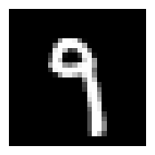
We might want to display multiple images at once. So, let’s create a subplots function next.
def subplots(
    nrows:int=1,
    ncols:int=1,
    figsize:tuple=None,
    imsize:int=3,
    suptitle:str=None,
    **kwargs
):
    "A figure and set of subplots to display images of `imsize` inches"
    if not figsize:
        # automatically calculate figure size if not given
        figsize=(ncols*imsize, nrows*imsize)

    fig,ax = plt.subplots(nrows, ncols, figsize=figsize, **kwargs)
    if suptitle is not None: fig.suptitle(suptitle)
    if nrows*ncols==1: ax = np.array([ax])
    return fig,ax
fig,axs = subplots(3,3, imsize=1)
imgs = xb[:8]
for ax,img in zip(axs.flat,imgs): show_image(img, ax)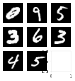
That’s a little ugly. Let’s do some clean up so we don’t have any of those leftover axes.
def get_grid(
    n:int,
    nrows:int=None,
    ncols:int=None,
    title:str=None,
    size:int=14,
    **kwargs,
):
    "Return a grid of `n` axes, `rows` by `cols`"
    # automatically calculate how many rows
    if nrows: ncols = ncols or int(np.floor(n/nrows))
    elif ncols: nrows = nrows or int(np.ceil(n/ncols))
    else:
        nrows = int(math.sqrt(n))
        ncols = int(np.floor(n/nrows))
    fig,axs = subplots(nrows, ncols, **kwargs)
    # turn off the axis for the leftovers
    for i in range(n, nrows*ncols): axs.flat[i].set_axis_off()
    if title: fig.suptitle(title, size=size)
    return fig,axs
fig,axs = get_grid(8, nrows=2, imsize=2)
for ax,img in zip(axs.flat,imgs): show_image(img, ax)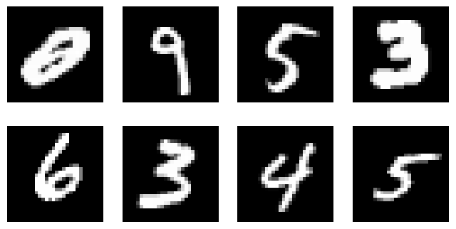
Finally let’s put the actual labels on the subplots as titles. It’s not the most useful here BUT it will be useful when working with random images that are not just MNIST.
from itertools import zip_longest

def show_images(ims:list,
                nrows:int|None=None,
                ncols:int|None=None,
                titles:list|None=None,
                **kwargs):
    "Show all images `ims` as subplots with `rows` using `titles`"
    # get_grid() returns a fig, axs and we only want the axs object
    axs = get_grid(len(ims), nrows, ncols, **kwargs)[1].flat
    for im,t,ax in zip_longest(ims, titles or [], axs): show_image(im, ax=ax, title=t)
from operator import itemgetter
lbls = yb[:8]
names = "0 1 2 3 4 5 6 7 8 9".split()
titles = itemgetter(*lbls)(names)?itemgetterInit signature: itemgetter(self, /, *args, **kwargs) Docstring: itemgetter(item, ...) --> itemgetter object Return a callable object that fetches the given item(s) from its operand. After f = itemgetter(2), the call f(r) returns r[2]. After g = itemgetter(2, 5, 3), the call g(r) returns (r[2], r[5], r[3]) File: /opt/conda/lib/python3.10/operator.py Type: type Subclasses:
itemgetter is a function that returns a function which lets us choose items from any object that has a __getitem__ so it can be a dict, list or whatever as long as the key (so the key in a dict or index in a list) is valid.
show_images(imgs[:8], imsize=1.7, titles=titles)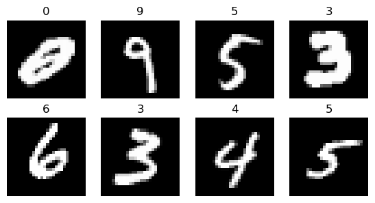
Refactored Training and Validation Loop
You always should also have a validation set, in order to identify if you are overfitting.
We will calculate and print the validation loss at the end of each epoch.
(Note that we always call model.train() before training, and model.eval() before inference, because these are used by layers such as nn.BatchNorm2d and nn.Dropout to ensure appropriate behaviour for these different phases.)
n_in, nh, n_out = x_train.shape[1], 50, y_train.max() + 1
n_in, nh, n_out
(784, 50, tensor(10))bs = 64
tds, vds = MNISTDataset(x_train, y_train), MNISTDataset(x_valid, y_valid)
tdl, vdl = DataLoader(tds, bs, shuffle=True, num_workers=2), DataLoader(vds, bs*2, shuffle=False)loss_func = F.cross_entropy
layers = [nn.Linear(n_in,nh), nn.ReLU(), nn.Linear(nh,n_out)]
model = nn.Sequential(*layers)
lr = 0.5
opt = optim.SGD(model.parameters(), lr=lr)def fit(model, tdl, vdl, opt, lossfunc, *args, lr, nepochs):
for epoch in range(nepochs):
model.train()
for xb, yb in tdl:
preds = model(xb)
loss = lossfunc(preds, yb)
loss.backward()
opt.step()
opt.zero_grad()
model.eval()
with torch.no_grad():
tot_loss, tot_acc, count = 0., 0., 0
for xb, yb in vdl:
preds = model(xb)
n = len(xb)
count += n
tot_loss += lossfunc(preds, yb).item() * n
tot_acc += accuracy(preds, yb).item() * n
print(epoch, tot_loss/count, tot_acc/count)
return tot_loss/count, tot_acc/countfit(model, tdl, vdl, opt, loss_func, lr=lr, nepochs=10)0 0.16485331418812274 0.9506
1 0.19638111138641834 0.9406
2 0.11045333566963672 0.9682
3 0.12151055069155992 0.965
4 0.10798258818089962 0.9693
5 0.1307273027807474 0.9615
6 0.1159135284371674 0.9702
7 0.10440870031602681 0.9732
8 0.7214727846324444 0.8906
9 0.10814986423365772 0.9724(0.10814986423365772, 0.9724)