Predicting the Partisanship of Politicians Through Analysis of Tweet-Specific Information
Introduction
Twitter is one of the most popular social media platforms, used for networking and micro-blogging where users post their thoughts in the form of tweets that can be maximum 280 characters long. As of 2019, Twitter has more than 330 million monthly active users with the US having the highest number of users of the platform. This wide level of usage leads to posts about various topics with news and politics being one of the major one and in fact Twitter was the largest source of breaking news during the U.S. Presidential Elections in 2016. This means that Twitter has a huge impact on the political sphere in the US and understanding the activities and discourses carried out by Democrats vs Republicans may help us use this information in many ways. Being able to judge orientation would be helpful in the organization of information into groups and make it easier for users to find and react to similar or opposite opinions thereby providing a better way to discuss and share information. This work presents investigation of the differences in tweets from users of the two different political preferences in the US. The differences in the tweets may reveal certain aspects that the individuals lean towards and may be useful for political leaders to use for future campaigns. The tweets we use in this analysis were provided to us and were not scraped. A total of N tweets can be found in the dataset - X of which are used for training and Y for testing. However, it must be drawn to the attention that the dataset used is very small when compared to the amount of political discourse that goes on in Twitter daily and hence our result may not be completely indicative of what kind of tweets are shared, liked, and posted by each party.
A first glance at the data tells us that there are a lot of entities in the text that need to be removed. So a preprocessing step is required. As we describe in Preprocessing, the preprocessing has a large implication on the accuracy of the classification and predictions. Both over-cleaning the data to remove important features and under-cleaning the data to keep features that can confuse the model lead to significantly lower accuracy as we will discuss.
With the cleaned and preprocessed text we then move on to understand our data better. We use techniques to understand target balance, i.e. whether there is a lot more data of one label relative to the other, ngram analysis to find the top 25 bi and trigrams by party, top 10 used hashtags by party, wordcloud, temporal evolution of retweets, favorites, and total tweets, and more. Descriptive Analysis details the processes used and visually summarizes the discoveries.
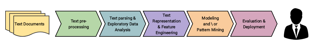
Finally, different features are extracted and various learning approaches are examined on the preprocessed data as we describe in Classification Methods. Various machine learning models such as Support Vector Machines, Logistic Regression, Ridge Classifier, Extreme Gradient Boosting (XGBoost), and Multinomial Naive Classifier are considered for the investigation. In addition we also consider cross-validation as well as hyperparameter tuning using GridSearch and Optuna. The overall contributions mentioned above are organized in following sections to come and the standard workflow for NLP projects as shown in Fig [fig:workflow] is followed.
Preprocessing
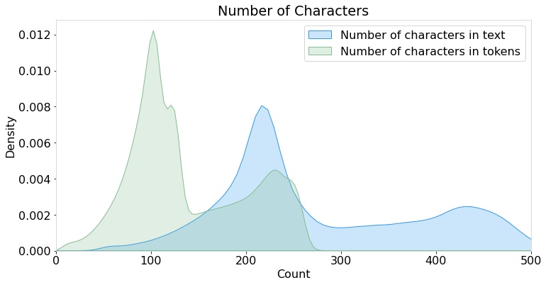
The preprocessing involves the use of the nltk module and regular expressions. First, a tokenization is carried out for each tweet to ensure appropriate parts-of-speech tagging. This step is important for lemmatization of the words to remove inflectional endings only and to return the base or dictionary form of the words. Once the tokens are lemmatized, stopwords, such as ‘are’, ‘we’, ‘is’, ‘am’ and all other English stopwords provided by the nltk module are removed. These processed tokens are then normalized. All punctuations, emojis, numbers, links, and as such are removed. In addition to these basic NLP cleaning procedure, tweet specific entities such as ‘RT’ and mentions are also removed. After these procedures are carried out, then any NaN values are replaced with empty strings. This concludes the preprocessing step leaving cleaned tweets for analysis. A plot of the relative lengths is shown in Fig [fig:lens] before and after cleaning.
Descriptive Analysis
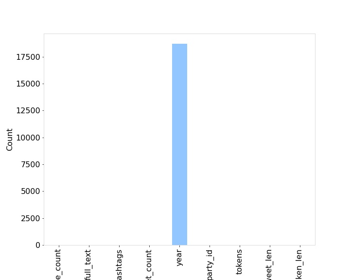
The dataset used had null values only for the year feature as shown below in Fig [fig:nullDistr]. As a result there was not a lot of null value corrections required.
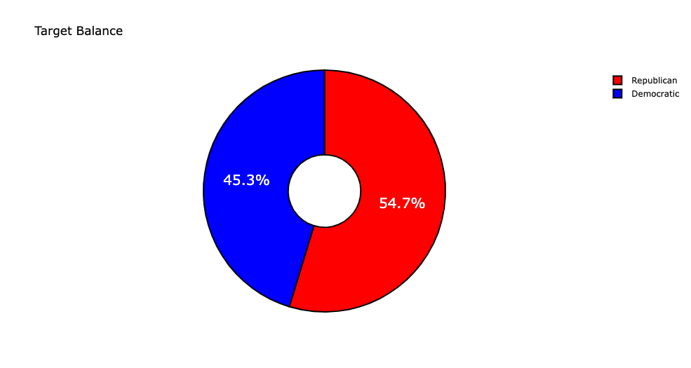
Next, the number of tweets labelled “R” and “D” were checked to ensure target balance. There was no significant imbalance in the dataset as shown in Fig [fig:imbalance] so no sampling was done for the rest of the process.
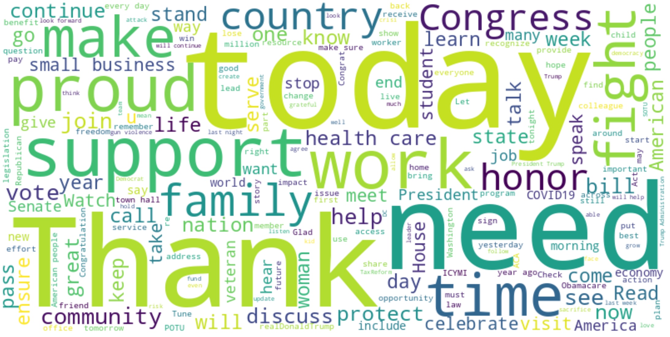
To explore whether the cleaned tweets are left with any noise, such as byte string, unicode characters or html entities, a wordcloud is generated as shown in Fig [fig:textcloud].
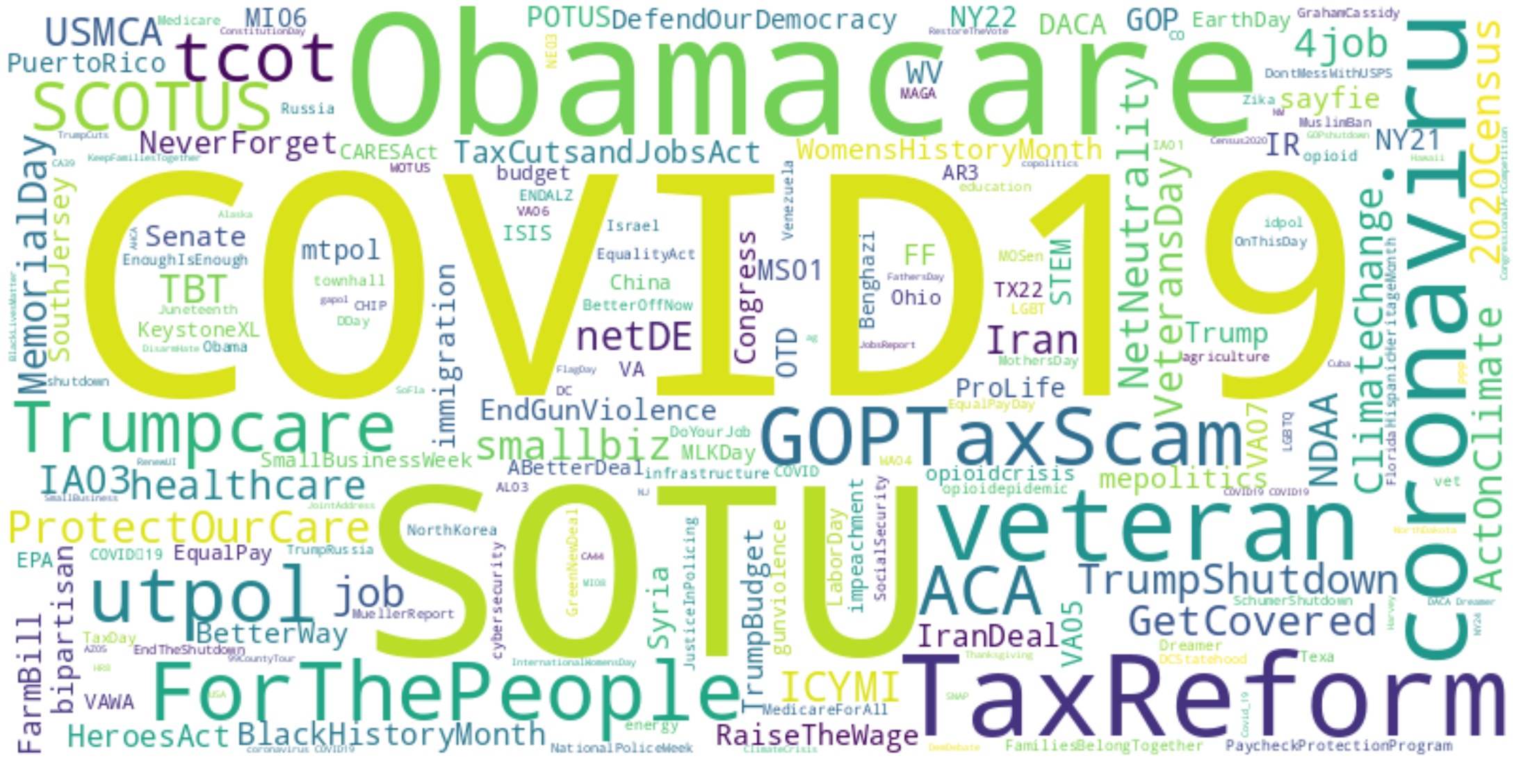
One of the main components that sets twitter apart from other social media are the hashtags. Some of the most used hashtags are visualized in Fig [fig:hashcloud].
The exploration of hashtags by party might reveal some patterns in the tweets themselves as a result barplot of the 10 most used hashtags is generated. While there are some similarities in the hashtags that are present for both parties, the frequencies vary vastly as can be seen in Fig [fig:top10hashtags]
.jpg)
However, from the plot there are many hashtags that are seen being highly used by the democrats relative to the republicans, such as, “ProtectOurCare” or “TrumpShutdown” and similar “TaxReform” can be seen twice in the plot for the republicans but never for the democrats. Such patterns will be useful when fitting the classification models and may be used as features alongside the cleaned tweets from Preprocessing.
As mentioned before, Fig. [fig:top10hashtags] shows shared usage of certain hashtags such as “COVID19.” To understand usage of certain words in context, ngrams can be very useful. As a result the top 25 bigrams and trigrams by party were also found and are summarized in Fig. [fig:bigrams] and [fig:trigrams].
.jpg)
.jpg)
While these bigrams and trigrams do not summarize the ideas into a category such as “COVID19” or “TaxReform” they will still provide insights on what type of ngram ranges to use when vectorizing the tweets for training.
Another feature specific to social media and Twitter are the favorite (or likes) and retweets (or shares) features. Such activities allow the tracing of interactions between users and their networks. Understanding how a tweet “performs” can allow better understanding of the interactions of users of the same political party with users within the party. As a result, the distribution of the top 1000 retweets and favorites by party are generated. Fig [fig:topfavs] and [fig:toprts] show how many of the top interactions were by republicans vs how many were by democrats.
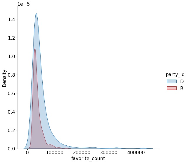
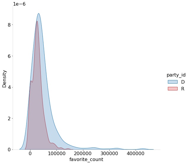
An imbalance in the number of favorite counts as well as retweet counts can be seen in the plots. In general it can be seen that the Democrats have higher retweet counts and favorite counts. It might also be interesting to see the time evolution of the counts instead of the dataset aggregate. As a result temporal behaviors are plotted in Fig [fig:temporal].
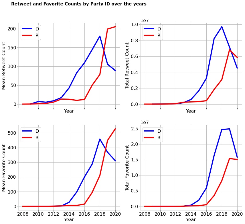
Just like the distribution, the temporal behavior also shows a more imbalanced distribution of retweets and favorites for the democrats in terms of total as well as mean. However, in the recent few years, Republicans do seem to have much higher mean retweets and favorite counts.
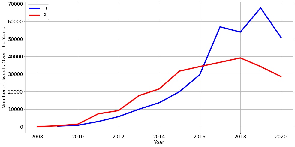
In terms of interactions it can also be useful to understand the total number of tweets over the years by party to understand which party has been more active on Twitter over the years. Fig. [fig:tempNum] shows that over the years the number of Democratic tweets have risen while the number of Republican tweets have fallen.
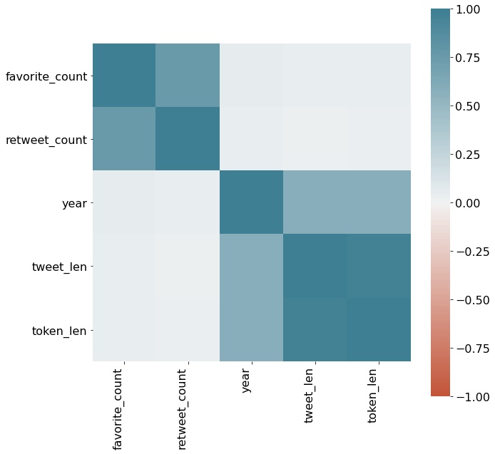
Finally, to understand whether there is a correlation between all the numerical data, a correlation matrix is constructed as shown in Fig [fig:corr]. The correlation matrix does show the trends we expect it to show as we have observed in all the other figures. Additionally it also shows that there is a positive correlation between the length of the raw tweets as well as the cleaned tweets over the years.
Feature Engineering and Extraction
Based on the observations drawn in exploratory data analysis, it was clear that data supplementary to the full tweet texts could be incorporated into the learning process. Namely, this information corresponded to the (per tweet) favorite count, retweet count, hashtags, character count, word count, hashtag count, mention count, mentions, and bigrams. Each of these extra information categories were extracted during data processing and supplanted as vectorized features into the datasets.
Each feature, barring those already in a numerical form, were vectorized using the term frequency–inverse document frequency (TF-IDF) vectorization scheme, which is a numerical statistic that reflects the relative significant of a word to a document. This statistic is computed through cascading the relative term frequency (TF) of a word with the inverse document frequency (IDF) weight - as laid out in .
Unfortunately, feature engineering with the additional metrics adds significant runtime and memory overhead since the feature space grows by an order of magnitude when doing so. However, this complexity hit is not entirely unwarranted since engineering features has shown to significantly improve classification results - as will be elaborated in the forthcoming section.
Classification Methods
In this section, the classification methods are discussed and described and in the following Classification Results the results for each are summarized and discussed.
Logistic Regression
One of the most common classifier models used for binary classification. The choice of implementing Logistic Regression was due to its simplicity as well as it’s ability to perform well for binary classifications. The model calculates the probability of a sample that belongs to a particular class by learning the set of parameters that minimize the induced log-likelihood over the training examples. The Logistic Regression model was also coupled with Cross-Validation techniques that are known to improve accuracy.
Ridge Classifier
The Ridge Classifier, which is based on Ridge regression, converts the labels into [-1, 1] and rephrases the problem into a regression problem thus enabling the use of regression methods. The highest value in prediction is accepted as a target class and for multiclass data muilti-output regression is applied. The Ridge Classifier was also coupled with Cross-Validation techiques.
Linear SVC
A discriminative classifier, also known as the Support Vector Classifier (SVC) is a machine learning algorithm derived from statistical learning theory based on the principle of structural risk minimization. It aims to reduce test error and computational complexity. The SVM identifies a separating hyper-plane with optimality between the two classes of a training dataset. This optimum separation is obtained by the hyper-plane that has the largest distance from the nearest training dataset. SVM techniques are known to be used for binary classification problems which is exactly what the current problem in question is.
Multinomial Naive Classifier
The Multinomial Naive Bayes algorithm is, as the name suggests, a Bayesian learning approach. The model guesses the label of a text using the Bayes theorem. It calculates each label’s likelihood for a given sample and outputs the label with the greatest probability. Just like the Naive Bayes Classifier, it too makes the naive assumption for independence among the features. The choice for the Mulinomial Classifier was once again made due to its simplicity as well as its popularity in known literature for NLP tasks.
XGBoost
XGBoost, which stands for Extreme Gradient Boosting, is a distributed gradient-boosted decision tree (GBDT) machine learning library. It provides parallel tree boosting and is the leading machine learning library for regression, classification, and ranking problems. We used the XGBoost Classifier for our classification problem. The XGBoost Classifier builds on the concepts of supervised machine learning, decision trees, ensemble learning, and gradient boosting. The choice of XGBoost was due to its well-known powerful nature. The XGBoost model with its large array of hyperparameters is often coupled with GridSearch or Optuna - a choice that was made even in this study.
Classification Results
This section summarizes the accuracy found from the models specified in Classification Methods in a descending order.
| Classifier | Accuracy % |
|---|---|
| Logistic Regression | 88.37 |
| Ridge Classifier | 88.15 |
| XGBoost | 88.00 |
| Linear SVC | 86.12 |
| Multinomial NB | 85.51 |
All these models were trained on the same feature vectors that were extracted using the method specified in Feature Engineering and Extraction. The simplest model among them all, Logistic Regression, consistently performed better. All the models were ran alongside K-fold cross-validation with 5 folds. The XGBoost tended to perform well on the training data but failed to perform well on the testing set, a characteristic behavior of a lot of tree methods. The Multinomial Naive Bayes classifier performed the worst. In terms of runtime the SVC model had the longest run-time followed by Multinomial NB and then XGBoost. Logistic Regression had the lowest runtime and performed the best.
CONCLUSIONS
To conclude, this work was to create a model that can classify tweets into two categories - Democrats and Republicans. The data was cleaned, examined, and features were extracted using known NLP techniques and libraries such as nltk, Tf-idf, matplotlib and as such. Multiple models were tested with Cross-validation Implementation as well as Hyperparameter Tuning methods for some. The model that performed the best was the Logistic Regression with parameters C=10 (and other default parameters) with the TF-IDF vectorization technique having an accuracy of 88.37%.