Introduction
In this post I will discuss the end-to-end implementation of a bear classifier and talk about the challenges that might come into play if one were to use even this extremely accurate model in a real system as well ways to mitigate those problems. One of the biggest obstacles with using deep learning methods for a problem is being able to keep an open eye to both the constraints that go into deep learning but also not underestimating how effective it can be. The recent rapid advancements definitely help with the latter, but, it is equally important to understand what exactly the model has learned and how its performance shifts as we show it more different types of data. But before that of course we need a model to begin with.
An End-to-End Application
The Drivetrain Approach
To create an end-to-end system, we need to first understand what goes into the entire project. Jeremy, Margit Zwemer, and Mike Loukides created a framework to think about this problem and named it “The Drivetrain Approach.” In order to effectively use deep learning, we should follow these in order:
- Objective: Define an objective or a problem statement we want to solve
- Lever: Understand what inputs that the objective is dependent on can we control
- Data: Understand what inputs we can even collect
- Models: How do our levers change our objective
Before we do the first three, we should not even think about building a model. So, let’s go through these in order.
Objective
Our goal is to create a model that can classify different bears so we can detect them in some camping site and figure out ways to keep them away. Interesting types of bears:
- Grizzly
- Polar
- Sloth
- Panda
- Tedd
Lever and Data
Well let’s say we can collect pictures of bears. We could use videos as well but for now let’s stick to something simpler and say we can get pictures of different types of bears. So, we can collect different images of some types of bears in different environments and build our model.
Models
We will be using some pretrained Computer Vision model.
Implementing the ideas
We will use some very similar tools as the previous blog post on Lesson and Chapter 1. Let’s import the libraries first.
from duckduckgo_search import ddg_images
from fastai.vision.all import *
from fastai.vision.widgets import *
from fastcore.all import *
I will explain as we go where we will be using each of these.
Collecting bear images from online
Let’s first download the images using ddg_images function from duckduckgo_search module and save them on our local storage.
def search_images(term: str, max_images: int = 30):
    print(f"Searching for {term}")
    images_json = ddg_images(term, max_images)
    return L(images_json).itemgot('image')


search_terms = 'grizzly', 'polar', 'sloth', 'panda', 'teddy'
path = Path("bears")

for term in search_terms:
    dest = path/term
    dest.mkdir(exist_ok=True, parents=True)
    download_images(dest, urls=search_images(f"{term} bear"))
    # resize the images as it takes a while to open large images
    resize_images(path=dest, max_size=400, dest=dest)
Deleting any corrupted images
When downloading files from the internet sometimes we can get corrupted files. We should remove them before we move on.
image_files = get_image_files(path)
failed = verify_images(image_files)
failed.map(Path.unlink)
This block of code gets the names of the image files, tries to open them and returns the ones that failed to open. Then we map the Path.unlink function over all the list of failed images so they are removed from our storage.
Building Datablock and Dataloaders
Let’s build a way to feed data into our model. This is the step of going from data -> dataloaders.
Create a Datablock
The Datablock class creates a template for our Dataloaders. We have already seen a Datablock in action in the previous post.
dblock = Datablock(
    blocks = (ImageBlock, CategoryBlock),
    get_items = get_image_files,
    get_y = parent_label,
    splitter = RandomSplitter(valid_pct=0.2),
    item_tfms = RandomResizedCrop(224, min_scale=0.5)
)
This has been explained at the end of the lesson 1 blog post: https://usiam.quarto.pub/fastai-lesson-blogs/posts/lesson_1/. Take a look at what each of the parameters are and what they represent!
A detour with Data Augmentations - item_tfms and batch_tfms
In certain projects, data can be hard to come by. In fact, even if there is data, it is very difficult and costly to label the data for supervised learning where you have your data and label and you create a model to learn the data and the labels. Data Augmentation techniques can help us reduce the problem of having little data to some extent. Another very important use case for Data Augmentation is that it allows our model to learn that rotating/stretching/flipping an image doesn’t change the fact that it still represents the same label i.e. a rotated/stretch/flipped car is still a car.
FastAI lets us do two types of transformations:
item_tfmson the CPU that are applied to all the itemsbatch_tfmson the GPU (if available) which are a lot faster and are applied to batches of data as theDataloadersfeed data into the model.
We can create a new blueprint with new transforms relative to the already existing dblock.
dblock = dblock.new(item_tfms=[RandomResizedCrop(128, min_scale=0.3)], batch_tfms=[*aug_transforms()])What we did here is create a new Datablock object from the exisiting one with new transforms applied. We kept everything else the same and just replaced the old transforms.
FastAI allows us various different ways to apply augmentations to data. Specifically, for images we have various options for item_tfms like cropping/squishing/padding/resizing and cropping etc. Some of these methods are:
item_tfms=Resize(128, ResizeMethod.Squish)item_tfms=Resize(128, ResizeMethod.Pad, pad_mode="zeros")item_tfms=RandomResizedCrop(128, min_scale=0.3)
It also provides us with different batch_tfms. Although, the recommended is to just use their aug_transforms().
You can also write your own transforms. That is covered in a future chapter.
Overall if you want to check out all the vision transformation options provided, check out the documentation: https://docs.fast.ai/vision.augment.html
Note: Vision transforms are not the only type of transformation possible. One EXTREMELY common transformation that is used is normalizaion and/or converting from Int to a Float tensor: batch_tfms = [IntToFloatTensor(), Normalize.from_stats(mean,std)].
Dataloaders
In fastai Dataloaders is a very thin class which essentially just stores a collection of Dataloader (notice the missing s) objects.
class DataLoaders(GetAttr):
    def __init__(self, *loaders):
        self.loaders = loaders
    def __getitem__(self, i):
        return self.loaders[i]

    # adds the two types by default using `add_props`
    train,valid = add_props(lambda i,self: self[i])
Using the Datablock class we can create different Dataloader objects which can then in turn create a Dataloaders object.
Let’s create the Dataloaders object from the dblock. It’s very easy. We already have the blueprint. All we need is to specify a path to actually get the data and a batch size to chunk the data.
dls = dblock.dataloaders(path, bs=32)
dls.train.show_batch(max_n=6) # shows 6 examples from the training set
dls.valid.show_batch(max_n=6) # shows 6 examples from the validation set
We have a way to feed data into our model while apply all sorts of transformations and whatnots to the data. Let’s create a Learner which is kind of a model grouped with a few other things.
Creating a Learner
The Learner class has also been explained in the first lesson’s post. Take a closer look.
learn = vision_learner(dls, 'resnet18', metrics=error_rate)
learn.fine_tune(4)
An application learner like vision_learner is a lot simpler than a non-application learner. We will build one of those in the next blog post on Lessons 3 & 5. For now all we need are the dataloaders object, the model type, and the metrics we want to use.
Because we are using a pretrained model like resnet18 we called .fine_tune(4) instead of something like .fit(4). The 4 here just represents the number of epochs/number of iterations over the entire dataset.
TIMM
This is a library of different image models maintained by Ross Wightman. It provides state-of-the-art (SOTA) pretrained CV models. To use timm we need to first install it using pip install timm and then import it.
import timm

timm.list_models('resnet*')
The above code returns a list of all CV models in timm that start with restnet. We can then choose one of them for our learner. Here’s a more thorough explanation of the timm library and comparisons using accuracy vs time plots for the different models of timm: https://www.kaggle.com/code/jhoward/which-image-models-are-best
Understanding the model performance
Let’s see where the model made mistakes during the classfication using some of the tools provided by the fastai library.
ClassificationInterpretation from vision.widgets will help us take a closer look at how our model is behaving. Specifically, we will take a look at two things: the confusion matrix and plots of images with the highest losses i.e. the images on which the model performed the worst.
Confusion Matrix
A confusion matrix is a grid of actual and predicted labels for all the classes in a binary/multiclass classification problem.
interp = ClassificationInterpretation.from_learner(learn)
interp.plot_confusion_matrix()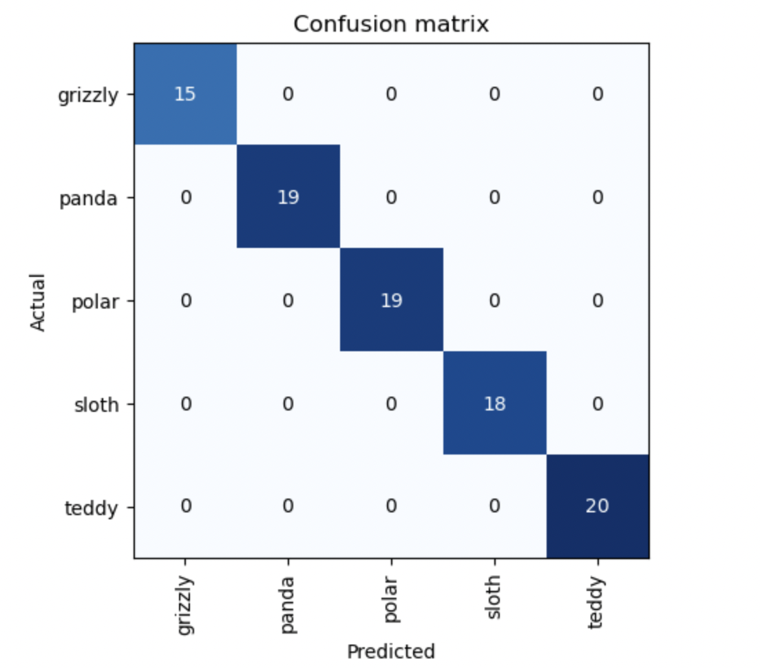
One thing we see here is, unfortunately (but not really), the classifier is actually perfect. It never makes a mistake. But sometimes for more difficult problems, we will see many numbers in the off diagonals that the actual label and the predicted labels were different thus lowering the accuracy of our model.
Images with high loss
This step can be very valuable in understanding what our model is struggling to learn. If we have some experts for the domain specific question, we can then show it to them and make certain hypothesis and test out different things we can do to help the learner learn these difficult images. We once again use the interpreter we instantiated above, interp to plot the images corresponding to top six highest losses.
interp.plot_top_losses(6)This will give us something that looks like this.
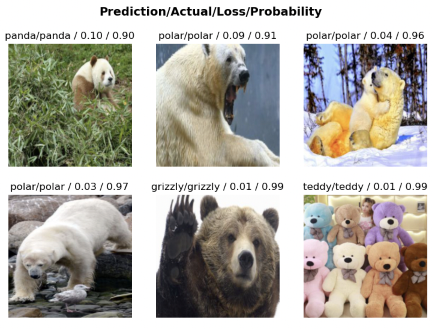
As the title says, for each image here we can see four pieces of information:
- What’s the predicted label?
- What’s the actual label?
- What’s the final loss?
- How confident is the label with its prediction?
Here, everything is perfect but we could use this information to say delete certain images that are maybe too blurry to learn from or some image where the subject is hidden behind something else.
Cleaning the data
Now that we’ve seen some of the images where the model did not perform well, let’s try to remove these “bad” images. Some very obvious images you would want to remove from the path are say images that may not have been bears or somehow a cartoon image of bear among many images of real bear pictures. Fastai provides some incredibly nice tools to clean your image data through the fastai.vision.widgets class. The one we will use is the ImageClassifierCleaner class which gives us a list of the images sorted in descending order of loss so we can inspect and remove “bad” images.
cleaner = ImageClassifierCleaner(learn)
cleaner
You should get an output that looks like this: 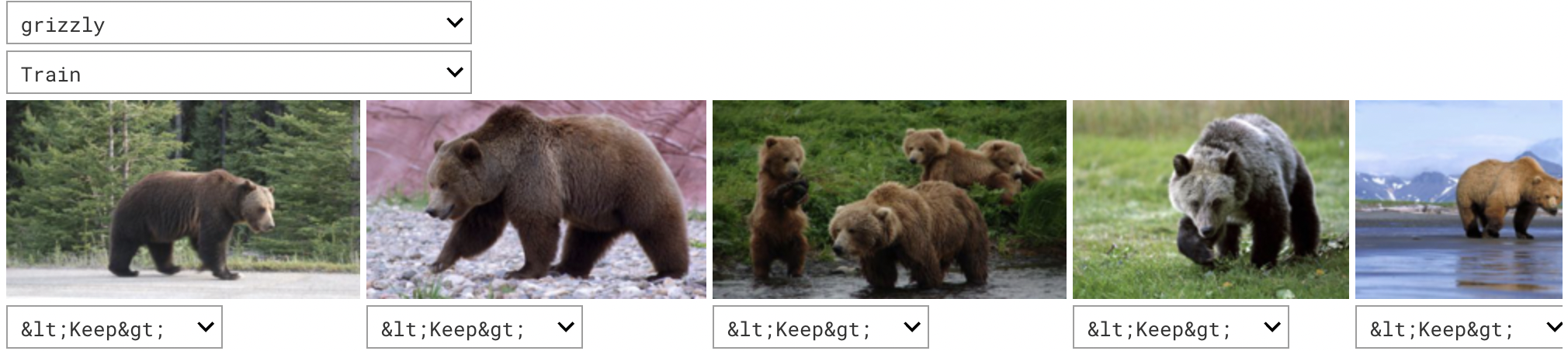
Now you can select what images you want to delete or move from both the training and validation datasets. Once you are happy with your selections you will modify the files with the following code:
for i in cleaner.delete():
    img_to_rm = cleaner.fns[i]
    img_to_rm.unlink()

for (i, category) in cleaner.change():
    from_path, to_path = str(cleaner.fns[i]), path/category
    shutil.move(from_path, to_path)
The cleaner object has access to the filenames as it contains the learner object. All we did in this block is (1) kept track of the files we want to delete, looped through them, and then just unlinked them (2) kept track of the files and corresponding categories we wanted to change, looped through them and then just moved them from old path to new path.
Retrain the model
Once we have finished cleaning up the data, we MUST create new dataloaders. Why? Well, if you remember, we have the dataloaders paths to the image files. But now some of those images don’t exist. If you try using the previous dataloaders objects, your program will crash. Let’s recreate the datablock, dataloaders, and learner with our newly cleaned up data.
dblock2 = DataBlock(
    blocks = (ImageBlock, CategoryBlock),
    get_items = get_image_files,
    get_y = parent_label,
    splitter = RandomSplitter(valid_pct = 0.2),
    item_tfms = [RandomResizedCrop(128, min_scale=0.3)],
    batch_tfms = [*aug_transforms()]
)

dls = dblock2.dataloaders(path, bs=32)

learn = vision_learner(dls, 'resnet18', metric=error_rate)
learn.fine_tune(4)
We now have our new trained model. We can iterate over these steps and clean more if we must. But let’s say we are now happy with our performance. Next thing to do is put it to use. What’s the point of a model that’s not used?
Save your model
Let’s save the model so we can load it somewhere else.
learn.export('model.pkl')Deployment
We will use gradio which is a tool provided by Huggingface. It allows us to deploy models that are hosted in their Huggingface Spaces.
The goal is to create a very simple interface right now where we upload an image and it tells us what the prediction is and how confident the model is. You can go crazy on deployment apps if you must but for now let’s stick to something basic and fast.
Create a classification function
Let’s first create a function that handles the classification logic before making the frontend.
def classify_images(img):
    learn = load_learner('model.pkl')
    categories = tuple(map(str.title, learn.dls.vocab))
    pred, indx, probs = learn.predict(img)
    return dict(zip(categories, map(float, probs)))
In order to ensure that the displayed categories are in the same order as the categories in the model, we want to automatically get the categories. That’s why we have the line: categories = tuple(map(str.title, learn.dls.vocab)). Another important line is the return line. The interface expects a dictionary of categories and corresponding probabilities. This is what the predict method’s return looks like:
learn.predict((path/'grizzly').ls()[0])

> ('grizzly', TensorBase(0), TensorBase([9.9414e-01, 2.2335e-04, 1.0752e-03, 2.5725e-04, 4.3061e-03]))
Using map we convert the TensorBase to a list of floats. The python idiom of dict(zip(x, y)) zips items in the two collections and uses the first item in each tuple as the key and the second item as the value. So finally we get something like this as our return:
dict(zip(categories, map(float, probs)))

> {'Grizzly': 0.9941380023956299,'Panda': 0.00022335126413963735,'Polar': 0.0010752034140750766,'Sloth': 0.00025724887382239103,'Teddy': 0.0043061161413788795}
Now let’s create the frontend interface.
Interface
We want some inputs, outputs, and optionally some example images. Then we want to provide our classify_images that will take in the input provided and return some output.
image = gr.inputs.Image(shape=(192, 192))
label = gr.outputs.Label()
examples = ["teddy.jpg", "panda.jpeg"]

intf = gr.Interface(fn=classify_image, inputs=image,
                    outputs=label, examples=examples)
intf.launch(inline=False)
This is what it will look like:
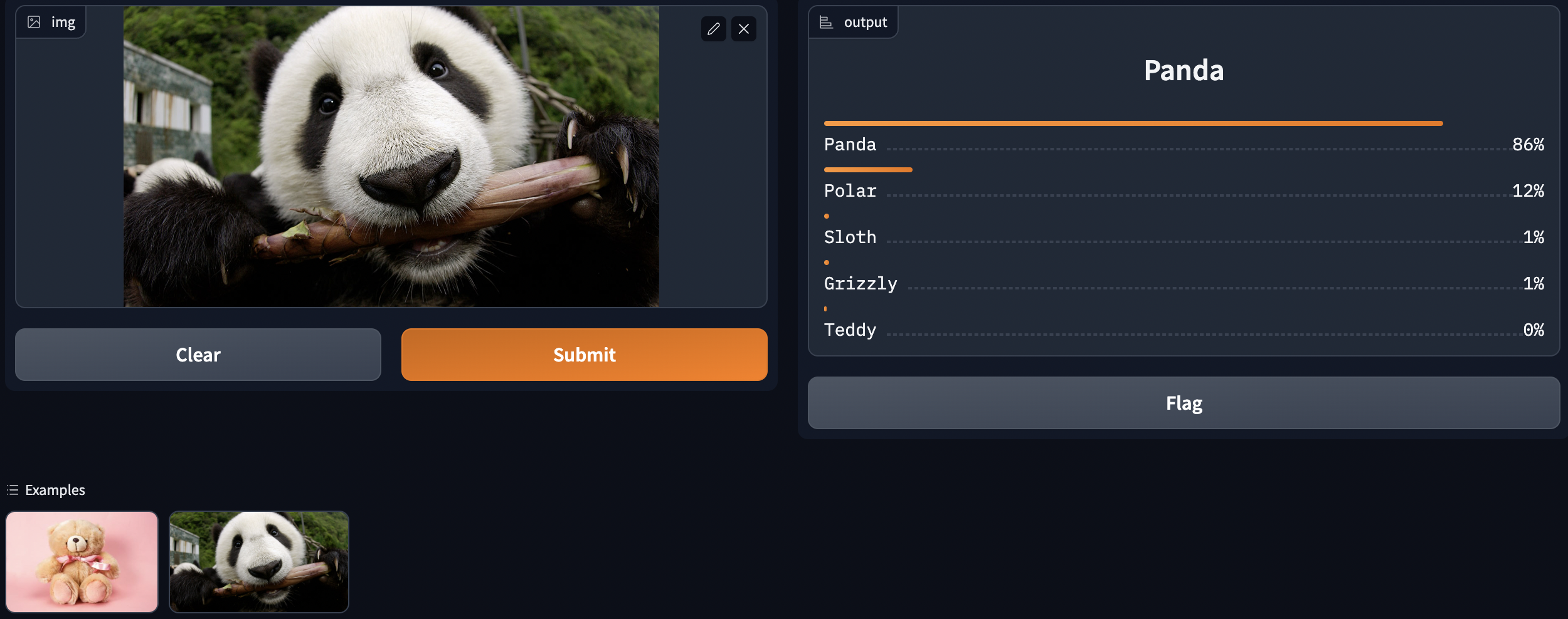
And we are done.
Problems with our very accurate model
Well we can now prevent bear attacks very easily with our fun little model. Or can we? You see in practice there are far too many things that can go wrong. The obvious one is, the images if you’ve noticed were very nice looking crisp high resolution pictures. If we were to monitor a camp-site we would be using CCTV cameras and they look awful. Additionally, we trained on images not videos. How would our model perform with that if we say took screenshots every t seconds. This brings us to two VERY important aspects of using deep learning (or honestly any) model in practice.
Out-of-Domain Data
Out-of-domain data is data that our model sees in production that is very different from what it was during training. For instance, blurry images at night were not present in the training nor validation data but might be what the model is performing inferences on in production. There is no complete technical solution to this problem; instead, we have to be careful about our approach to rolling out the technology.
Domain or Data Shift
Domain shift is where the type of data that our model sees changes over time. For instance, an insurance company may use a deep learning model as part of its pricing and risk algorithm, but over time the types of customers the company attracts and the types of risks it represents may change so much that the original training data is no longer relevant.
Avoiding Disasters Systematically
Out-of-domain data and domain shift are examples of a larger problem: that you can never fully understand all the possible behaviors of a neural network, because they have far too many parameters. In other words, the strongest thing about neural networks is also their weakness. Let’s try to figure out a systematic approach to mitigating this issue.
Manual Process: This is the first step in rolling out these technologies. EVERYTHING that the model predicts is carefully checked by some human. This is so we can monitor how exactly the model is behaving and what are the things it’s getting wrong IN PRODUCTION.
Limited Scope Development: This is the second step. In this step we are a little more comfortable with relying on the model so we deploy and monitor it in a limited scope say in one national park every 4 hours for a month.
Gradual Expansion: This step is a natural progression from the next. We slowly expand our deployments to more and more scopes such as all national parks in a state and monitor it every day. During the expansion, it is very important to ensure that you have really good reporting systems in place, to make sure that you are aware of any signifi‐ cant changes to the actions being taken compared to your manual process. For instance, if the number of bear alerts doubles or halves after rollout of the new system in some location, you should be very concerned.
Following these high-level steps and thinking more deeply about the use cases of your model will help avoid as many problems as possible. One of the most important things to take away from this section is that the “end-to-end” system does not stop after the deployment. In fact, that’s when it is truly important to monitor and understand the behaviors of the model and continuously making changes to it when necessary.
Conclusions
In this blog post we saw a way to approach problems using deep learning based solutions with The Drivetrain Approach. We also look at an end-to-end classification system and deployed it. We also looked at the challenges of using models in production in the form of out-of-domain data and domain shift. Finally we talked about a high level approach to slowly automate these processes with human-in-the-loop feedback before completely relying on them.
Here’s the accompanying Kaggle notebook for this blog post: https://www.kaggle.com/code/usiam04/fastai-pt1-lec02